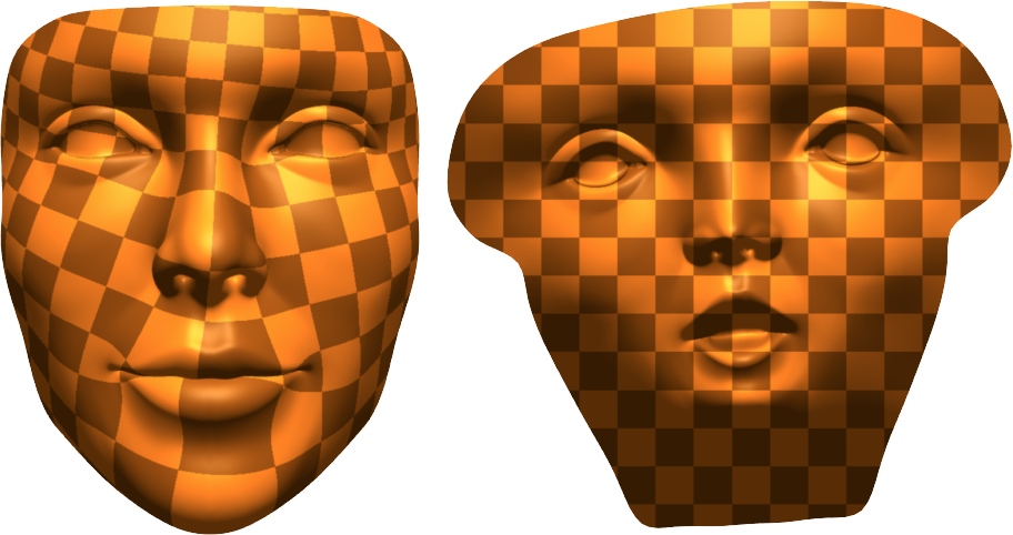
Assignment 4: Conformal Parameterization
The written part of your next assignment, on conformal surface parameterization, can be found here. Conformal parameterization is useful for (among many other things) finding maps between cortical surfaces, or designing shape-shifting matter. You’ll have the opportunity to implement one of these algorithms in the coding part of the assignment.

For the coding portion of your assignment, you will implement the Spectral Conformal Parameterization (SCP) algorithm, which is detailed in the course notes.
Please implement the following routines in
- core/geometry.[js/cpp]:
- complexLaplaceMatrix
- projects/parameterization/spectral-conformal-parameterization.[js/cpp]:
- buildConformalEnergy
- flatten
- utils/solvers.[js/cpp]:
- solveInversePowerMethod
- residual
- The complex version of the cotan-Laplace matrix can be built in exactly the same manner as its real counterpart. The only difference now is that the cotan values of our matrix will be complex numbers with a zero imaginary component. This time, we will work with meshes with boundary, so your Laplace matrix will have to handle boundaries properly (you just have to make sure your cotan function returns 0 for halfedges which are in the boundary).
- The buildConformalEnergy function builds a \(|V| \times |V|\) complex matrix corresponding to the conformal energy \(E_C(z) = E_D(z) - \mathcal A(Z)\) where \(E_D\) is the Dirichlet energy (given by our complex cotan-Laplace matrix) and \(\mathcal A\) is the total signed area of the region \(z(M)\) in the complex plane (Please refer to Section 7.4 of the notes for more details). You may find it easiest to iterate over the halfedges of the mesh boundaries to construct the area matrix (Recall that the Mesh object has a boundaries variable which stores all the boundary loops.
- The flatten function returns a dictionary mapping each vertex to a vector (linear-algebra/vector.js) of planar coordinates by finding the eigenvector corresponding to the smallest eigenvalue of the conformal energy matrix. You can compute this eigenvector by using solveInversePowerMethod (described below).
- Your solveInversePowerMethod function should implement Algorithm 1 in Section 7.5 of the course notes with one modification – after computing \(Ay_i = y_{i-1}\), center \(y_i\) around the origin by subtracting its mean. You don't have to worry about the \(B\) matrix or generalized eigenvalue problem. Important: Terminate your iterations when your residual is smaller than \(10^{-10}\).
- The parameterization project directory also contains a basic implementation of the Boundary First Flattening (BFF) algorithm. Feel free to play around with it in the viewer and compare the results to your SCP implementation.