Assignment 4 [Coding]: Conformal Parameterization (Due 5/6)

For the coding portion of your assignment on conformal parameterization, you will implement the Spectral Conformal Parameterization (SCP) algorithm as described in the course notes.Please implement the following routines in

  1. core/geometry.[js|cpp]:
    1. complexLaplaceMatrix
  2. projects/parameterization/spectral-conformal-parameterization.[js|cpp]:
    1. buildConformalEnergy
    2. flatten
  3. utils/solvers.[js|cpp]:
    1. solveInversePowerMethod
    2. residual

Notes

  • Warning: In the notes, the residual is defined as the vector $Ax – \lambda x$. But your function residual  should return a float. You should return $\frac{\|Ax – \lambda x\|_2}{\|x\|_2}$. Furthermore, you should compute $\lambda$ as $\frac{x^* Ax}{x^* x}$ where $x^*$ is the conjugate transpose of $x$.
  • The complex version of the cotan-Laplace matrix can be built in exactly the same manner as its real counterpart. The only difference now is that the cotan values of our matrix will be complex numbers with a zero imaginary component. This time, we will work with meshes with boundary, so your Laplace matrix will have to handle boundaries properly (you just have to make sure your cotan function returns 0 for halfedges which are in the boundary).
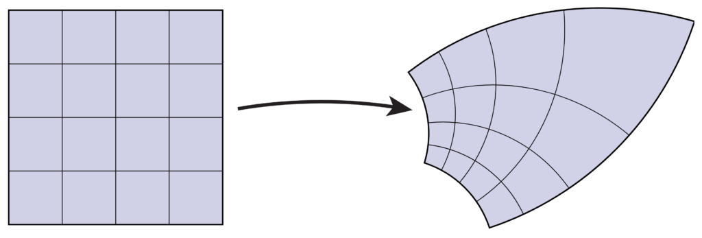
  • The buildConformalEnergy function builds a $|V| \times |V|$ complex matrix corresponding to the conformal energy $E_C(z) = E_D(z) – \mathcal A(Z)$ where $E_D$ is the Dirichlet energy (given by our complex cotan-Laplace matrix) and $\mathcal A$ is the total signed area of the region $z(M)$ in the complex plane (Please refer to Section 7.4 of the notes for more details). You may find it easiest to iterate over the halfedges of the mesh boundaries to construct the area matrix (Recall that the Mesh object in the JS framework has a boundaries variable which stores all the boundary loops; similarly in Geometry Central you can iterate directly over boundary loops.)
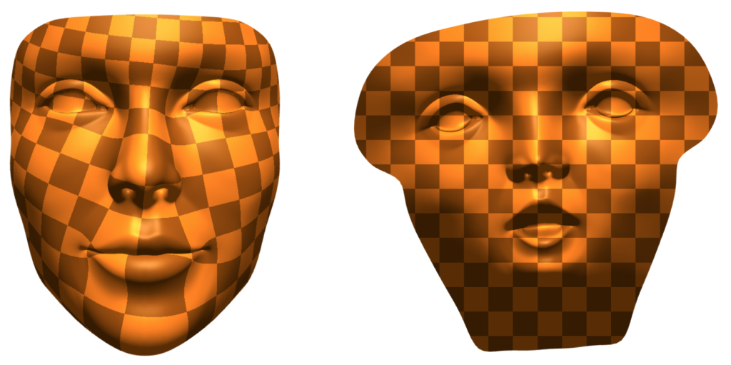
  • The flatten function returns a dictionary mapping each vertex to a vector of planar coordinates by finding the eigenvector corresponding to the smallest eigenvalue of the conformal energy matrix. You can compute this eigenvector by using solveInversePowerMethod (described below).
  • Your solveInversePowerMethod function should implement Algorithm 1 in Section 7.5 of the course notes with one modification – after computing $Ay_i = y_{i-1}$, center $y_i$ around the origin by subtracting its mean. You don’t have to worry about the $B$ matrix or generalized eigenvalue problem. Important: Terminate your iterations when your residual is smaller that 10^-10.
  • The parameterization project directory also contains a basic implementation of the Boundary First Flattening (BFF) algorithm. Feel free to play around with it in the viewer and compare the results to your SCP implementation.

Submission Instructions

Please submit your source files to the course Gradescope by 5:59pm ET.

Assignment 4 [Written]: Conformal Parameterization (Due 5/6)


The written part of your next assignment, on conformal surface flattening, is now available below. Conformal flattening is important for (among other things) making the connection between processing of 3D surfaces, and existing fast algorithms for 2D image processing. You’ll have the opportunity to implement one of these algorithms in the coding part of the assignment.


Assignment 4

Reading 7—Discrete Conformal Geometry (Due 5/3)

Your next reading will take a deep dive into conformal geometry and the many ways to discretize and compute conformal maps. This subject makes some beautiful and unexpected connections to other areas of mathematics (such as circle packings, and hyperbolic geometry), and is in some sense one of the biggest “success stories” of DDG, since there is now a complete uniformization theorem that mirrors the one on the smooth side. You’ll find out more about what this all means in the reading! The reading comes from the note, “Conformal Geometry of Simplicial Surface”:


For your assignment you will need to read the Overview (1.1) and Preliminaries (1.2); you must also pick one of Part I, Part II, or Part III to read, each of which covers a different perspective on discrete conformal maps. The most interesting subject, perhaps, is the connections to hyperbolic geometry in Part IV, which you can read for your own enjoyment! 🙂

Hand-in instructions are, as usual, found on the assignments page. The reading is due at 10 AM Eastern, May 3, 2021.

Lectures 19 & 20: Conformal Geometry

A basic task in geometric algorithms is finding mappings between surfaces, which can be used to transfer data from one place to another. A particularly nice class of algorithms (both from a mathematical and computational perspective) are conformal mappings, which preserve angles between vectors, and are generally very well-behaved. In this lecture we’ll take a look at smooth characterizations of conformal maps, which will ultimately inspire the way we talk about conformal maps in the discrete/computational setting.

The video covering both today and Thursday’s lecture (on discrete aspects of conformal maps) can be found here.

Lecture 18: The Laplace-Beltrami Operator

In this lecture we take a close look at the Laplacian, and its generalization to curved spaces via the Laplace-Beltrami operator. The Laplacian is one of the most fundamental objects in geometry and physics, and which plays a major role in algorithms. Here we consider several perspectives to build up some basic intuition about what the Laplacian is, and what it means.

Lecture 17—Discrete Curvature II (Variational Viewpoint)

In this lecture we wrap up our discussion of discrete curvature, and see how it all fits together into a single unified picture that connects the integral viewpoint, the variational viewpoint, and the Steiner formula. Along the way we’ll touch upon several of the major players in discrete differential geometry, including a discrete version of Gauss-Bonnet, Schläfli’s polyhedral formula, and the cotan Laplace operator—which will be the focus of our next set of lectures.

Lecture 16—Discrete Curvature I (Integral Viewpoint)

Just as curvature provides powerful ways to describe and analyze smooth surfaces, discrete curvatures provide a powerful way to encode and manipulate digital geometry—and is a fundamental component of many modern algorithms for surface processing. This first of two lectures on discrete curvature from the integral viewpoint, i.e., integrating smooth expressions for discrete curvatures in order to obtain curvature formulae suitable for discrete surfaces. In the next lecture, we will see a complementary variational viewpoint, where discrete curvatures arise by instead taking derivatives of discrete geometry. Amazingly enough, these two perspectives will fit together naturally into a unified picture that connects essentially all of the standard discrete curvatures for triangle meshes.

Assignment 3 [Coding]: The Laplacian (Due 4/22)

For the coding portion of this assignment, you will build the so-called “cotan-Laplace” matrix and start to see how it can be used for a broad range of surface processing tasks, including the Poisson equation and two kinds of curvature flow.


Getting Started

Please implement the following routines in

  1. core/geometry.[cpp|js]:
    • laplaceMatrix
    • massMatrix
  2. projects/poisson-problem/scalar-poisson-problem.[cpp|js]:
    • constructor
    • solve
  3. projects/geometric-flow/mean-curvature-flow.[cpp|js]:
    • buildFlowOperator
    • integrate
  4. projects/geometric-flow/modified-mean-curvature-flow.[cpp|js]:
    • constructor
    • buildFlowOperator


Notes

  • Sections 6.4-6 of the course notes describe how to build the cotan-Laplace matrix and mass matrices, and outline how they can be used to solve equations on a mesh. In these applications you will be required to setup and solve a linear system of equations $Ax=b$ where $A$ is the Laplace matrix, or some slight modification thereof. Highly efficient numerical methods such as Cholesky Factorization can be used to solve such systems, but require A to be symmetric positive definite. Notice that the cotan-Laplace matrix described in the notes is negative semi-definite. To make it compatible for use with numerical methods like the Cholesky Factorization, your implementation of laplaceMatrix should instead produce a positive definite matrix, i.e., it should represent the expression
    $$(\Delta u)_i=\frac12 \sum_{ij}(\cot \alpha_{ij}+\cot \beta_{ij})(u_i–u_j).$$(Note that $u_i−u_j$ is reversed relative to the course notes.) To make this matrix strictly positive definite (rather than semidefinite), you should also add a small offset such as $10^{-8}$ to the diagonal of the matrix (which can be expressed in code as a floating point value 1e-8). This technique is known as Tikhonov regularization.
  • The mass matrix is a diagonal matrix containing the barycentric dual area of each vertex.
  • In the scalar Poisson problem, your goal is to discretize and solve the equation $\Delta \phi = \rho$ where $rho$ is a scalar density on vertices and $\Delta$ is the Laplace operator. Be careful about appropriately incorporating dual areas into the discretization of this equation (i.e., think about where and how the mass matrix should appear); also remember that the right-hand side cannot have a constant component (since then there is no solution).
  • In your implementation of the implicit mean curvature flow algorithm, you can encode the surface $f:M \to \mathbb R^3$ as a single DenseMatrix of size $|V| \times 3$, and solve with the same (scalar) cotan-Laplace matrix used for the previous part. When constructing the flow operator, you should follow section 6.6 of the notes. But be careful – when we discretize equations of the form $\Delta f = \rho$, we create systems of the form $A f = M \rho$. So you’ll need to add in the mass matrix somewhere. Also, recall that our discrete Laplace matrix is the negative of the actual Laplacian.
  • The modified mean curvature flow is nearly identical to standard mean curvature flow. The one and only difference is that you should not update the cotan-Laplace matrix each time step, i.e., you should always be using the cotans from the original input mesh. The mass matrix, however, must change on each iteration.


Submission Instructions

Please only turn in the source files geometry.[cpp|js], scalar-poisson-problem.[cpp|js], mean-curvature-flow.[cpp|js] and modified-mean-curvature-flow.[cpp|js] . These files should be submitted via the usual mechanism, as described on the assignments page.

Assignment 3 [Written]: The Laplacian (Due 4/22)

These exercises will lead you through two different derivations for the cotan-Laplace operator. As we’ll discuss in class, this operator is basically the “Swiss army knife” of discrete differential geometry and digital geometry processing, opening the door to a huge number of interesting algorithms and applications. Note that this time the exercises all come from the course notes—you will need to read the accompanying notes in order to familiarize yourself with the necessary material (we’ll cover some of this stuff in greater depth later on, but you don’t need it for the assignment!)


Reading 6—The Laplace Operator (due April 15)

Your next reading covers one of the most fundamental objects in differential geometry, and one of the most useful objects in practical geometry processing: the Laplace-Beltrami operator \(\Delta\), which we’ll often refer to as just the “Laplacian”. This operator generalizes the familiar Laplace operator \(\Delta = \frac{\partial^2}{\partial x_1^2} + \cdots + \frac{\partial^2}{\partial x_n^2}\) from Euclidean \(\mathbb{R}^n\) to general curved manifolds. Like the ordinary Laplacian, at a very basic level Laplace-Beltrami provides information about the “curvature” of a function. It also shows up in an enormous number of physical and geometric equations, and for this reason there has been intense study of different ways to discretize the Laplacian (not only for simplicial meshes, but also point clouds and other discrete surface representations).

The next written assignment will give you some essential background on the smooth Laplace operator. This reading will also expose you to some of the key issues to think about when designing a discrete Laplacian. For this reading, you can choose either of the following two papers:

You should not worry about deeply understanding all of the mathematical details in these papers; the point is just to get a sense of the issues at stake, and how these considerations translate into practical definitions of discrete Laplace matrices. The first paper, by Wardetzky et al, considers a “No Free Lunch” theorem for discrete Laplacians that continues our story of “The Game” played in discrete differential geometry. The second paper, by Bobenko & Springborn considers the important perspective of intrinsic triangulations of polyhedral surfaces, and uses this perspective to develop a Laplace operator that is well-behaved even for very poor quality triangulations. You should simply summarize the high-level ideas in these papers, and any questions you might have.

The reading is due on Thursday, April 15 at 10am Eastern time. Hand-in instructions are as usual described on the assignments page.