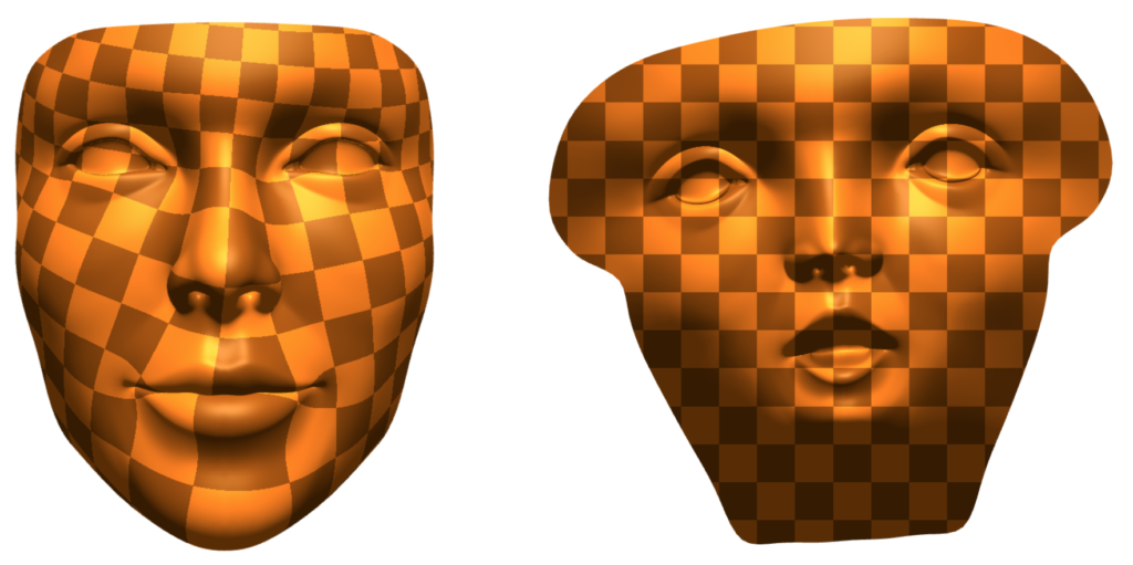
For the coding portion of your assignment on conformal parameterization, you will implement the Spectral Conformal Parameterization (SCP) algorithm as described in the course notes.Please implement the following routines in
- core/geometry.js:
- complexLaplaceMatrix
- projects/parameterization/spectral-conformal-parameterization.js:
- buildConformalEnergy
- flatten
- utils/solvers.js:
- solveInversePowerMethod
- residual
Notes
- I added a few tests for utils/solvers.js. They’re available in the git repository. If you’re familiar with git, you can pull the changes. If you’d prefer not to mess around with git, you can also just download the files and put them in tests/utils.
- Warning: I fixed a problem with the residual test. In the notes, the residual is defined as a vector $Ax – \lambda x$. But your function residual should return a float. You should return $\frac{\|Ax – \lambda x\|_2}{\|x\|_2}$. Furthermore, you should compute $\lambda$ as $\frac{x^\dagger A x}{x^\dagger x}$ where $x^\dagger$ is the conjugate transpose of $x$.
- The complex version of the cotan-Laplace matrix can be built in exactly the same manner as its real counterpart. The only difference now is that the cotan values of our matrix will be complex numbers with a zero imaginary component. This time, we will work with meshes with boundary, so your Laplace matrix will have to handle boundaries properly (you just have to make sure your cotan function returns 0 for halfedges which are in the boundary).
- The buildConformalEnergy function builds a $|V| \times |V|$ complex matrix corresponding to the conformal energy $E_C(z) = E_D(z) – \mathcal A(Z)$ where $E_D$ is the Dirichlet energy (given by our complex cotan-Laplace matrix) and $\mathcal A$ is the total signed area of the region $z(M)$ in the complex plane (Please refer to Section 7.4 of the notes for more details). You may find it easiest to iterate over the halfedges of the mesh boundaries to construct the area matrix (Recall that the Mesh object has a boundaries variable which stores all the boundary loops.
- The flatten function returns a dictionary mapping each vertex to a vector (linear-algebra/vector.js) of planar coordinates by finding the eigenvector corresponding to the smallest eigenvalue of the conformal energy matrix. You can compute this eigenvector by using solveInversePowerMethod (described below).
- Your solveInversePowerMethod function should implement Algorithm 1 in Section 7.5 of the course notes with one modification – after computing $Ay_i = y_{i-1}$, center $y_i$ around the origin by subtracting its mean. You don’t have to worry about the $B$ matrix or generalized eigenvalue problem. Important: Terminate your iterations when your residual is smaller that 10^-10.
- The parameterization project directory also contains a basic implementation of the Boundary First Flattening (BFF) algorithm. Feel free to play around with it in the viewer and compare the results to your SCP implementation.
Submission Instructions
Please rename your geometry.js, spectral-conformal-parameterization.js and solvers.js files to geometry.txt, spectral-conformal-parameterization.txt and solvers.txt (respectively) and put them in a single zip file called solution.zip. These files and your solution to the written exercises should be submitted together in a single email to Geometry.Collective@gmail.com with the subject line DDG19A4.

In the third “Notes” bullet point, in “…corresponding to the conformal energy $E_C(z) = E_D(z) – A(z)$ where $?_?$ is the Dirichlet energy…” is it $E_D$ is the Dirichlet energy?
Yes, sorry for the typo. It should be fixed now.
I don’t quite understand how flatten() would return a dictionary mapping each vertex to a vector of planar coordinates. What do we do after finding the eigenvector of the smallest eigenvalue of the conformal energy matrix? Would we need to multiply the vertex positions by the appropriate entry of that eigenvector?
Each entry of the eigenvector is a complex number, which you can think of as a point in the plane. Explicitly, each vertex should be mapped to a vector whose x coordinate is the real part of the complex number, and whose y coordinate is the imaginary part.
Thanks!
When I was implementing the “residual” function, I am literally using $Ax-\lambda x$ with $\lambda = x^T Ax$ to find the residual and returning $\frac{\|Ax-\lambda x\|_2}{\| x \|_2}$. However, I am not passing the test case for residual. Is there anything that we need to be careful about? I called residual in my solveInversePowerMethod function, and that works fine.
I have the same issue. My residual worked for the old test script, but now when I simply take the norm the numbers do not even closely match. Is there something special about taking the norm in this case?
Sorry, the formula that I wrote down for lambda only works for unit vectors. You should compute $\lambda$ as $\frac{x^\dagger A x}{x^\dagger x}$ (where $x^\dagger$) is the conjugate transpose. I’ll fix the writeup above.
The signature for Solvers.residual() requires us to return a number. However, the test
let error = computed_residual.minus(expected_residual).norm(2);
seems to treat what the function returns as a complexDenseMatrix, and a type error occurs. Should we return a complexDenseMatrix instead?
I updated the test file in the git repo to take in a number instead of a complexDenseMatrix. Do you have the newest version of the test?
Oh I didn’t pull the newest changes. Sorry!
How do we test our complexLaplaceMatrix function? I don’t see any tests for it.
Sorry, there aren’t any tests for it – just the test for your conformal energy.
I plugged the matrix for the solveInversePowerMethod test into matlab and it looks like the solution eigen vector is the one to the second lowest eigen value. Should we be trying to get second eigen, or did I do something wrong?
Your solveInversePowerMethod should compute the first non-constant eigenvector. Subtracting the mean off of your vector each iteration projects out any constant component of your vector. Since the first eigenvector of matrix in the test is constant, your function should return the second eigenvector of this matrix.
Got it. When I subtract the mean I pass the test and I was getting the constant vector. Thanks!