CS 15-458/858: Discrete Differential Geometry

Warning: You cannot use late days on this assignment since it’s the last one.

In this assignment, you will investigate tools for working with tangent vector fields on surfaces. Tangent vector fields are central to classical differential geometry, and have many interesting applications. For this homework, we’ll look at one algorithm for designing vector fields, and along the way we’ll cover a lot of deep facts about surfaces.

There’s no PDF this week since the exercises are all from the notes.

Do any 12 of Exercise 8.1 – Exercise 8.21 in the notes, except for Exercise 8.13.

Submission Instructions. Please submit your solutions to the exercises (whether handwritten, LaTeX, etc.) as a single PDF file by email to Geometry.Collective@gmail.com. This email must also contain the .zip file for your coding solution. Scanned images/photographs can be converted to a PDF using applications like Preview (on Mac) or a variety of free websites (e.g., http://imagetopdf.com). Your submission email must include the string DDG19A6 in the subject line.

Warning: You cannot use late days on this assignment since it’s the last one.

Warning: You cannot use late days on this assignment since it’s the last one.

Please implement the following routines in:

1. projects/vector-field-decomposition/tree-cotree.js:
   1. buildPrimalSpanningTree
   2. inPrimalSpanningTree
   3. buildDualSpanningCotree
   4. inDualSpanningCotree
   5. buildGenerators
2. projects/vector-field-decomposition/harmonic-bases.js:
   1. buildClosedPrimalOneForm
   2. compute

In addition, please implement either Hodge Decomposition, or Trivial Connections (on surfaces of genus 0):

Hodge Decomposition: Please implement the following routines in

1. projects/vector-field-decomposition/hodge-decomposition.js:
   1. constructor
   2. computeExactComponent
   3. computeCoExactComponent
   4. computeHarmonicComponent

Trivial Connections on Surfaces of Genus 0: Please implement computeConnections in projects/direction-field-design/trivial-connections.js. This file has function signatures for trivial connections on arbitrary surfaces, but for this assignment we are only requiring you to compute the connection form on simply-connected surfaces where you don’t have to worry about the period matrix. You are, of course, welcome to implement the general algorithm if you would like to!

Notes:

• I made some changes to the tests for this assignment, and to the trivial connections viewer. You should update the following files before starting the assignment:
  • tests/vector-field-decomposition/test.html
  • tests/vector-field-decomposition/test.js
  • tests/direction-field-design/sphere.js
  • tests/direction-field-design/test.html
  • tests/direction-field-design/test.js
  • projects/direction-field-design/index.html
• Recall that homology generators are a set of loops which somehow describe all of the interesting loops on a surface. For example, here are the two homology generators for the torus.
• Your buildGenerators function should implement the Tree-Cotree algorithm, which is Algorithm 5 of section 8.2 of the notes.
• In tree-cotree.js the trees are stored using the dictionaries vertexParent and faceParent. You should store the primal spanning tree by storing the parent of vertex v in vertexParent[v]. The root should be its own parent. Similarly, you should store the dual spanning cotree by storing the parent of face f in faceParent[f].
• The Tree Cotree algorithm finds homology generators on the dual mesh. That is to say, you should take each dual edge which is not in either spanning tree, and form a loop by following its endpoint back up the dual cotree until they meet at the root of the dual cotree. Even though we’re thinking of these homology generators as loops on the dual mesh, we still store them as lists of ordinary halfedges, since edges in the dual mesh are in 1-1 correspondence with edges in the primal graph.
• buildClosedPrimalOneForm should use a homology generator to construct a closed primal 1-form as described in section 8.22 of the notes.
• The compute function in HarmonicBases should compute a harmonic basis using Algorithm 6 in section 8.2 of the notes. If you choose to implement Hodge decomposition for the assignment, you are welcome to use your Hodge decomposition code to solve for $d\alpha$. Otherwise, you can just ignore the hodgeDecomposition parameter and directly solve the linear system $\Delta \alpha = \delta \omega$ to find $\alpha$. (Recall that $\delta$ is the codifferential, which we talked a lot about in the Discrete Exterior Calculus assignment).

Notes (Hodge Decomposition):

• The procedure for Hodge Decomposition is given as Algorithm 3 in section 8.1 of the Notes.
• Note that the SparseMatrix class has an invertDiagonal function that you can use to invert diagonal matrices.
• For computeCoExactComponent, you should compute the coexact component $\delta \beta$ of a differential form $\omega$ by solving the equation $d\delta \beta = d\omega$. As stated in the notes, the most convenient way of doing this is to define a dual 0-form $\tilde \beta := *\beta$, and then to solve $d*d \tilde \beta = d \omega$. Then you can compute $\delta \beta$ using the fact that $\delta \beta = *d*\beta = *d\tilde\beta$. When doing these computations, you should keep tract of whether your forms are primal forms or dual forms, recalling that hodge stars take you from primal forms to dual forms, and hodge star inverses take you from dual forms to primal forms. (THis is discussed in detail in section 8.1.3 of the notes.
• Note that the 2-form Laplacian B is not necessarily positive definite, so you should use an LU solver instead of a Cholesky solver when solving systems involving B.

Notes (Trivial Connections):

• The trivial-connection-js file is structured for implementing the full trivial connections algorithm on arbitrary surfaces. Since that’s tricky, we’re only requiring that you compute connections on topological spheres. You should implement this in the computeConnections() function, and it should pass the tests labeled “computeConnections on a sphere”.
• Even though we’re working with spheres, it is still helpful to use the formulation of Trivial connections given in section 8.4.1 of the notes. In particular, you should solve the optimization problem given in Exercise 8.21.
• On a sphere, there are no harmonic 1-forms, so the $\gamma$ part of your Hodge decomposition will always be 0. Furthermore, the sphere has no homology generators, so the problem simplifies to \[\min_{\delta \beta} \;\|\delta\beta\|^2\;\text{s.t.}\; d\delta\beta = u\]
• Following the notes, we observe that the constraint $d\delta\beta = u$ determines $\beta$ up to a constant, and that constant is annihilated by $\delta$. So you can find the connection 1-form $\delta \beta$ with a single linear solve.

Submission Instructions
Please rename all js files you edited to be txt files and put them in a single zip file called solution.zip. This file and your solution to the written exercises should be submitted together in a single email to Geometry.Collective@gmail.com with the subject line DDG19A6.

Warning: You cannot use late days on this assignment since it’s the last one.

Here’s the writeup for your second to last assignment. This time, we’re taking off the “training wheels” and having you read a real paper, rather than course notes. Why? Because you’re ready for it! At this point you have all the fundamental knowledge you need to go out into the broader literature and start implementing all sorts of algorithms that are built on top of ideas from differential geometry. In fact, this particular algorithm is not much of a departure from things you’ve done already: solving simple equations involving the Laplacian on triangle meshes. As discussed in our lecture on the Laplacian, you’ll find many algorithms in digital geometry processing that have this flavor: compute some basic data (e.g., using a local formula at each vertex), solve a Laplace-like equation, compute some more basic data, and so on.

Your main references for this assignment will be:

• this video, which gives a brief (18-minute) overview of the algorithm, and
• this paper, which explains the algorithm in detail.

Written exercises for this assignment are found below.

For the coding portion of this assignment, you will implement the heat method, which is an algorithm for computing geodesic distance on curved surfaces. All of the details you need for implementation are described in Section 3 of the paper, up through and including Section 3.2. Note that you need only be concerned with the case of triangle meshes (not polygon meshes or point clouds); pay close attention to the paragraph labeled “Choice of Timestep.”

Please implement the following routines in:

1. projects/geodesic-distances/heat-method.js:
   1. constructor
   2. computeVectorField
   3. computeDivergence
   4. compute

Notes

• Refer to sections 3.2 of the paper for discretizations of Algorithm 1 (page 3).
• Recall that our Laplace matrix is positive semidefinite, which might differ from the sign convention the authors use.
• The tests for computeVectorField and computeDivergence depend on the A and F matrices you define in your constructor. So if you fail the tests but your functions look correct, check whether you have defined the flow and laplace matrices properly.
• Your solution should implement zero neumann boundary conditions (which are the “default behavior” of the cotan Laplacian) but feel free to tryout other Dirichlet and Neumann boundary conditions on your own.

Submission Instructions

Please rename your heat-method.js file to heat-method.txt and put it in a single zip file called solution.zip. This file and your solution to the written exercises should be submitted together in a single email to Geometry.Collective@gmail.com with the subject line DDG19A4.

The written part of your next assignment, on conformal surface flattening, is now available below. Conformal flattening is important for (among other things) making the connection between processing of 3D surfaces, and existing fast algorithms for 2D image processing. You’ll have the opportunity to implement one of these algorithms in the coding part of the assignment.

These exercises will lead you through two different derivations for the cotan-Laplace operator. As we’ll discuss in class, this operator is basically the “Swiss army knife” of discrete differential geometry and digital geometry processing, opening the door to a huge number of interesting algorithms and applications. Note that this time the exercises all come from the course notes—you will need to read the accompanying notes in order to familiarize yourself with the necessary material (though actually we’ve covered much of this stuff in class already!)

The written portion of Assignment 2 can be found below. It takes a look at the curvature of smooth and discrete surfaces, which we have been talking about in lecture. Note that you are required to complete only two problems from each section!

Warning: We renumbered the Exercises in the course notes to make more sense, so you make sure you refer to the updated notes when doing these exercises.

For the coding portion of this assignment, you will implement various expressions for discrete curvatures and surfaces normals that you will derive in the written assignment. (However, the final expressions are given below in case you want to do the coding first.) Once implemented, you will be able to visualize these geometric quantities on a mesh. For simplicity, you may assume that the mesh has no boundary.

Getting Started
Please implement the following routines in core/geometry.js:

1. angle
2. dihedralAngle
3. vertexNormalAngleWeighted
4. vertexNormalSphereInscribed
5. vertexNormalAreaWeighted
6. vertexNormalGaussianCurvature
7. vertexNormalMeanCurvature
8. angleDefect
9. totalAngleDefect
10. scalarMeanCurvature
11. circumcentricDualArea
12. principalCurvatures

Notes 

1. The dihedral angle between the normals $N_{ijk}$ and $N_{ijl}$ of two adjacent faces $ijk$ and $ijl$ (respectively) is given by
$$ \theta_{ij} := \text{atan2}\left(\frac{e_{ij}}{\|e_{ij}\|} \cdot \left(N_{ijk} \times N_{jil}\right), N_{ijk} \cdot N_{jil}\right)$$

where $e_{ij}$ is the vector from vertex $i$ to vertex $j$.

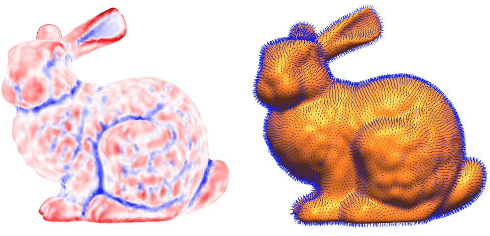
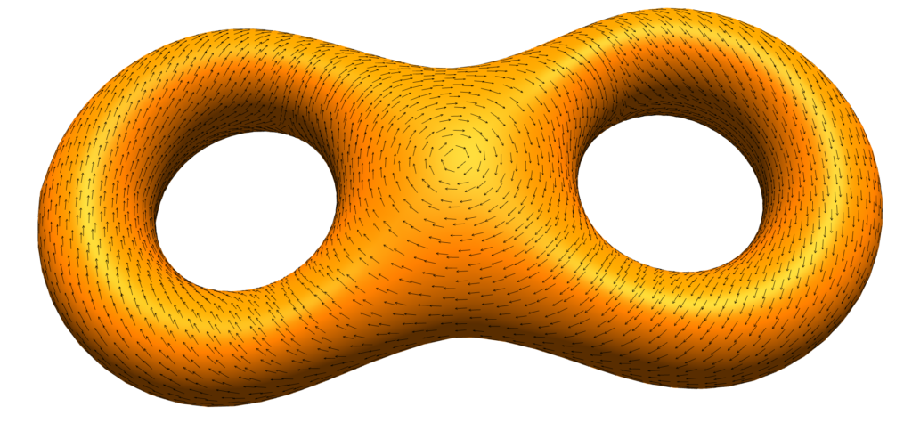
2. The formulas for the angle weighted normal, sphere inscribed normal, area weighted normal, discrete Gaussian curvature normal and discrete mean curvature normal at vertex $i$ are
\[\begin{aligned}
N_i^\phi &:= \sum_{ijk \in F} \phi_i^{jk}N_{ijk}\\
N_i^S &:= \sum_{ijk \in F} \frac{e_{ij} \times e_{ik}} {\|e_{ij}\|^2\|e_{ik}\|^2}\\
N_i^A &:= \sum_{ijk \in F} A_{ijk}N_{ijk}\\
KN_i &= \frac 12 \sum_{ij \in E} \frac{\theta_{ij}}{\|e_{ij}\|}e_{ij}\\
HN_i &= \frac 12 \sum_{ij \in E}\left(\cot\left(\alpha_k^{ij}\right) + \cot\left(\beta_l^{ij}\right)\right)e_{ij}
\end{aligned}
\]

where $\phi_i^{jk}$ is the interior angle between edges $e_{ij}$ and $e_{ik}$, and $A_{ijk}$ is the area of face $ijk$. Note that sums are taken only over elements (edges or faces) containing vertex $i$. Normalize the final value of all your normal vectors before returning them.

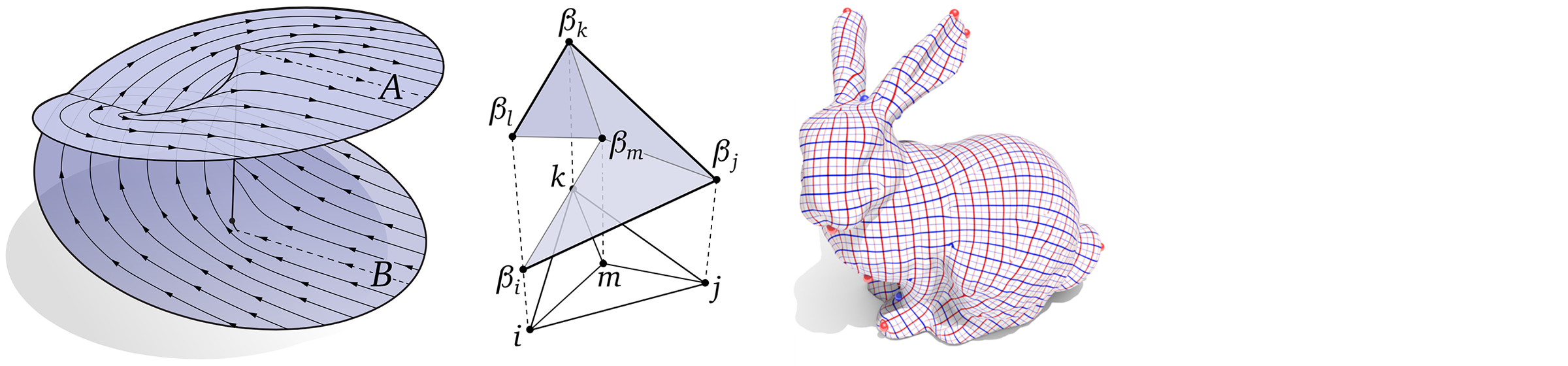
3. The circumcentric dual area at vertex $i$ is given by
\[A_i := \frac 18 \sum_{ijk \in F} \|e_{ik}\|^2\cot\left(\alpha_j^{ki}\right) + \|e_{ij}\|^2\cot\left(\beta_k^{ij}\right)\]

4. The discrete scalar Gaussian curvature (also known as angle defect) and discrete scalar mean curvature at vertex $i$ are given by
\[\begin{aligned}
K_i &:= 2\pi – \sum_{ijk \in F} \phi_i^{jk}\\
H_i &:= \frac 12 \sum_{ij \in E} \theta_{ij}\|e_{ij}\|
\end{aligned}
\]

Note that these quantities are discrete 2-forms, i.e., they represent the total Gaussian and mean curvature integrated over a neighborhood of a vertex. They can be converted to pointwise quantities (i.e., discrete 0-forms at vertices) by dividing them by the  circumcentric dual area of the vertex (i.e., by applying the discrete Hodge star).

5. You are required to derive expressions for the principal curvatures $\kappa_1$ and $\kappa_2$ in exercise 4 of the written assignment. Your implementation of principalCurvatures should return the (pointwise) minimum and maximum principal curvature values at a vertex (in that order).

Submission Instructions

Please rename your geometry.js file to geometry.txt and put it in a single zip file called solution.zip. This file and your solution to the written exercises should be submitted together in a single email to Geometry.Collective@gmail.com with the subject line DDG19A2.

For the coding portion of your first assignment, you will implement the discrete exterior calculus (DEC) operators $\star_0, \star_1, \star_2, d_0$ and $d_1$. Once implemented, you will be able to apply these operators to a scalar function (as depicted above) by pressing the “$\star$” and “$d$” button in the viewer. The diagram shown above will be updated to indicate what kind of differential k-form is currently displayed. These basic operations will be the starting point for many of the algorithms we will implement throughout the rest of the class; the visualization (and implementation!) should help you build further intuition about what these operators mean and how they work

Getting Started

• For this assignment, you need to implement the following routines:
  1. in core/geometry.js
     1. cotan
     2. barycentricDualArea
  2. in core/discrete-exterior-calculus.js
     1. buildHodgeStar0Form
     2. buildHodgeStar1Form
     3. buildHodgeStar2Form
     4. buildExteriorDerivative0Form
     5. buildExteriorDerivative1Form

In practice, a simple and efficient way to compute the cotangent of the angle $\theta$ between two vectors $u$ and $v$ is to use the cross product and the dot product rather than calling any trigonometric functions directly; we ask that you implement your solution this way. (Hint: how are the dot and cross product of two vectors related to the cosine and sine of the angle between them?)

In case we have not yet covered it in class, the barycentric dual area associated with a vertex $i$ is equal to one-third the area of all triangles $ijk$ touching $i$.

EDIT: You can compute the ratio of dual edge lengths to primal edge lengths using the cotan formula, which can be found on Slide 28 of the Discrete Exterior Calculus lecture, or in exercise 36 of the notes (you don’t have to do the exercise for this homework).

Submission Instructions

Please rename your geometry.js and discrete-exterior-calculus.js files to geometry.txt and discrete-exterior-calculus.txt (respectively) and submit them in a single zip file called solution.zip by email to Geometry.Collective@gmail.com.

The written portion of assignment 1 is now available (below), which covers some of the fundamental tools we’ll be using in our class. Initially this assignment may look a bit intimidating, but keep a few things in mind:

• The homework is not as long as it might seem: all the text in the big gray blocks contains supplementary, formal definitions that you do not need to know in order to complete the assignments.
• Moreover, note that you are required to complete only three problems from each section.

Finally, don’t be shy about asking us questions here in the comments, via email, or during office hours.  We want to help you succeed on this assignment, so that you can enjoy all the adventures yet to come…

This assignment is due on Tuesday, February 26.

For the written part of your first homework you will do some exercises that will help familiarize you with basic descriptions and representations of combinatorial surfaces (simplicial surfaces, adjacency matrices, halfedge meshes), which will help prepare you to work with such surfaces as we continue through the course. (If any of this stuff seems abstract right now, don’t worry: we’ll use it over and over again to implement “real” algorithms starting in just a couple weeks!)

You must complete 8 out of 15 exercises in the Written Exercises section of Chapter 2 of the course notes. You may choose any set of 8 exercises you like, but if you do more than 8, please mark clearly on your submission which ones you would like us to grade.

The assignment is due on February 7, 2019 at 5:59:59pm Eastern (not at midnight!). Further hand-in instructions can be found on this page.

For the coding portion of your first assignment, you will implement some operations on simplicial complexes which were discussed in class and in Chapter 2 of the course notes. Once implemented, you will be able to select simplices and apply these operations to them by clicking the appropriate buttons in the viewer (shown above).

Getting Started

• Please download or clone the files in this repository. It contains a fast and flexible framework for 3D geometry processing implemented in Javascript. Over the course of the semester, you will implement all of your coding assignments here.
• For this assignment, you will need to implement the following routines in projects/simplicial-complex-operators/simplicial-complex-operators.js:
  • assignElementIndices
  • buildVertexEdgeAdjacencymatrix
  • buildEdgeFaceAdjacencymatrix
  • buildVertexVector
  • buildEdgeVector
  • buildFaceVector
  • star
  • closure
  • link
  • isComplex
  • isPureComplex
  • boundary

Notes

• This assignment comes with a viewer projects/simplicial-complex-operators/index.html which lets you apply your operators to simplices of meshes and visualize the results.
• Selecting simplices will not work until you fill in the assignElementIndices function.
• The assignment also comes with a test script tests/simplicial-complex-operators/text.html which you can use to verify the correctness of your operators.
• The code framework is implemented in Javascript, which means no compilation or installation is necessary on any platform. You can simply get started by opening the index.html file in projects/discrete-exterior-calculus/ in a web browser. We recommend using Chrome or Firefox. Safari has poor WebGL performance.
• If you do not have prior experience with Javascript, do not worry! You should be able to get a handle on Javascript syntax by reading through some of the code in the framework (a good place to start might be core/geometry.js). The framework also contains extensive documentation (see docs/index.html).
• All browsers come with tools for debugging (for instance the JavaScript Console in Chrome).

Submission Instructions

Please rename your simplicial-complex-operators.js file to simplicial-complex-operators.txt and submit it in a zip file called solution.zip to Geometry.Collective@gmail.com.