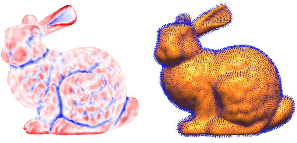
Assignment 6 [Written]: Vector Field Decomposition and Design (Due 5/14)

Warning: You cannot use late days on this assignment since it’s the last one.

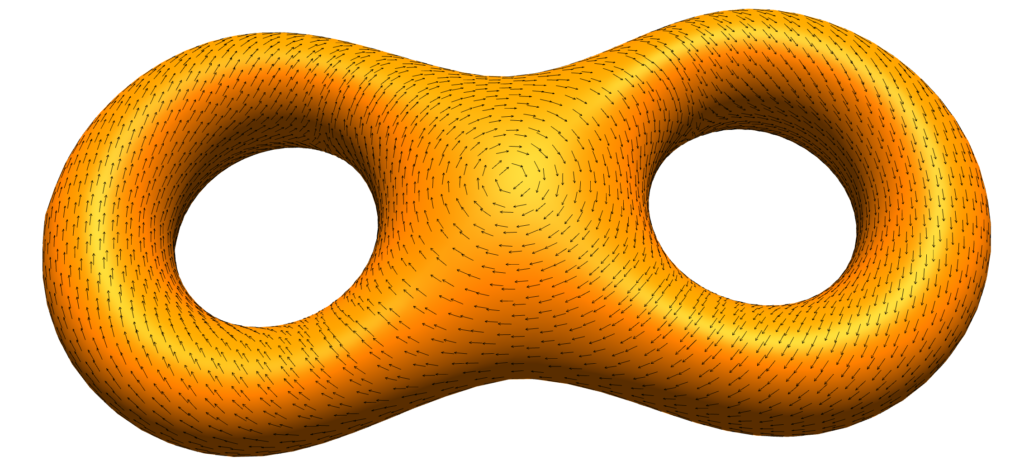
In this assignment, you will investigate tools for working with tangent vector fields on surfaces. Tangent vector fields are central to classical differential geometry, and have many interesting applications. For this homework, we’ll look at one algorithm for designing vector fields, and along the way we’ll cover a lot of deep facts about surfaces.

There’s no PDF this week since the exercises are all from the notes.

Do any 12 of Exercise 8.1 – Exercise 8.21 in the notes, except for Exercise 8.13.

Submission Instructions. Please submit your solutions to the exercises (whether handwritten, LaTeX, etc.) as a single PDF file by email to Geometry.Collective@gmail.com. This email must also contain the .zip file for your coding solution. Scanned images/photographs can be converted to a PDF using applications like Preview (on Mac) or a variety of free websites (e.g., http://imagetopdf.com). Your submission email must include the string DDG19A6 in the subject line.

Warning: You cannot use late days on this assignment since it’s the last one.

Assignment 6 [Coding]: Vector Field Decomposition and Design (Due 5/14)

Warning: You cannot use late days on this assignment since it’s the last one.

Please implement the following routines in:

  1. projects/vector-field-decomposition/tree-cotree.js:
    1. buildPrimalSpanningTree
    2. inPrimalSpanningTree
    3. buildDualSpanningCotree
    4. inDualSpanningCotree
    5. buildGenerators
  2. projects/vector-field-decomposition/harmonic-bases.js:
    1. buildClosedPrimalOneForm
    2. compute

In addition, please implement either Hodge Decomposition, or Trivial Connections (on surfaces of genus 0):

Hodge Decomposition: Please implement the following routines in

  1. projects/vector-field-decomposition/hodge-decomposition.js:
    1. constructor
    2. computeExactComponent
    3. computeCoExactComponent
    4. computeHarmonicComponent

Trivial Connections on Surfaces of Genus 0: Please implement computeConnections in projects/direction-field-design/trivial-connections.js. This file has function signatures for trivial connections on arbitrary surfaces, but for this assignment we are only requiring you to compute the connection form on simply-connected surfaces where you don’t have to worry about the period matrix. You are, of course, welcome to implement the general algorithm if you would like to!

Notes:

  • I made some changes to the tests for this assignment, and to the trivial connections viewer. You should update the following files before starting the assignment:
    • tests/vector-field-decomposition/test.html
    • tests/vector-field-decomposition/test.js
    • tests/direction-field-design/sphere.js
    • tests/direction-field-design/test.html
    • tests/direction-field-design/test.js
    • projects/direction-field-design/index.html
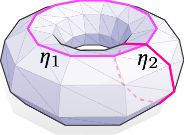
  • Recall that homology generators are a set of loops which somehow describe all of the interesting loops on a surface. For example, here are the two homology generators for the torus.
  • Your buildGenerators function should implement the Tree-Cotree algorithm, which is Algorithm 5 of section 8.2 of the notes.
  • In tree-cotree.js the trees are stored using the dictionaries vertexParent and faceParent. You should store the primal spanning tree by storing the parent of vertex v in vertexParent[v]. The root should be its own parent. Similarly, you should store the dual spanning cotree by storing the parent of face f in faceParent[f].
  • The Tree Cotree algorithm finds homology generators on the dual mesh. That is to say, you should take each dual edge which is not in either spanning tree, and form a loop by following its endpoint back up the dual cotree until they meet at the root of the dual cotree. Even though we’re thinking of these homology generators as loops on the dual mesh, we still store them as lists of ordinary halfedges, since edges in the dual mesh are in 1-1 correspondence with edges in the primal graph.
  • buildClosedPrimalOneForm should use a homology generator to construct a closed primal 1-form as described in section 8.22 of the notes.
  • The compute function in HarmonicBases should compute a harmonic basis using Algorithm 6 in section 8.2 of the notes. If you choose to implement Hodge decomposition for the assignment, you are welcome to use your Hodge decomposition code to solve for $d\alpha$. Otherwise, you can just ignore the hodgeDecomposition parameter and directly solve the linear system $\Delta \alpha = \delta \omega$ to find $\alpha$. (Recall that $\delta$ is the codifferential, which we talked a lot about in the Discrete Exterior Calculus assignment).

Notes (Hodge Decomposition):

  • The procedure for Hodge Decomposition is given as Algorithm 3 in section 8.1 of the Notes.
  • Note that the SparseMatrix class has an invertDiagonal function that you can use to invert diagonal matrices.
  • For computeCoExactComponent, you should compute the coexact component $\delta \beta$ of a differential form $\omega$ by solving the equation $d\delta \beta = d\omega$. As stated in the notes, the most convenient way of doing this is to define a dual 0-form $\tilde \beta := *\beta$, and then to solve $d*d \tilde \beta = d \omega$. Then you can compute $\delta \beta$ using the fact that $\delta \beta = *d*\beta = *d\tilde\beta$. When doing these computations, you should keep tract of whether your forms are primal forms or dual forms, recalling that hodge stars take you from primal forms to dual forms, and hodge star inverses take you from dual forms to primal forms. (THis is discussed in detail in section 8.1.3 of the notes.
  • Note that the 2-form Laplacian B is not necessarily positive definite, so you should use an LU solver instead of a Cholesky solver when solving systems involving B.

Notes (Trivial Connections):

  • The trivial-connection-js file is structured for implementing the full trivial connections algorithm on arbitrary surfaces. Since that’s tricky, we’re only requiring that you compute connections on topological spheres. You should implement this in the computeConnections() function, and it should pass the tests labeled “computeConnections on a sphere”.
  • Even though we’re working with spheres, it is still helpful to use the formulation of Trivial connections given in section 8.4.1 of the notes. In particular, you should solve the optimization problem given in Exercise 8.21.
  • On a sphere, there are no harmonic 1-forms, so the $\gamma$ part of your Hodge decomposition will always be 0. Furthermore, the sphere has no homology generators, so the problem simplifies to \[\min_{\delta \beta} \;\|\delta\beta\|^2\;\text{s.t.}\; d\delta\beta = u\]
  • Following the notes, we observe that the constraint $d\delta\beta = u$ determines $\beta$ up to a constant, and that constant is annihilated by $\delta$. So you can find the connection 1-form $\delta \beta$ with a single linear solve.

Submission Instructions
Please rename all js files you edited to be txt files and put them in a single zip file called solution.zip. This file and your solution to the written exercises should be submitted together in a single email to Geometry.Collective@gmail.com with the subject line DDG19A6.

Warning: You cannot use late days on this assignment since it’s the last one.

Assignment 5 [Written]: Geodesic Distance (Due 5/2)

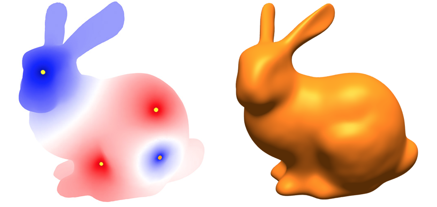
Here’s the writeup for your second to last assignment. This time, we’re taking off the “training wheels” and having you read a real paper, rather than course notes. Why? Because you’re ready for it! At this point you have all the fundamental knowledge you need to go out into the broader literature and start implementing all sorts of algorithms that are built on top of ideas from differential geometry. In fact, this particular algorithm is not much of a departure from things you’ve done already: solving simple equations involving the Laplacian on triangle meshes. As discussed in our lecture on the Laplacian, you’ll find many algorithms in digital geometry processing that have this flavor: compute some basic data (e.g., using a local formula at each vertex), solve a Laplace-like equation, compute some more basic data, and so on.

Your main references for this assignment will be:

  • this video, which gives a brief (18-minute) overview of the algorithm, and
  • this paper, which explains the algorithm in detail.

Written exercises for this assignment are found below.


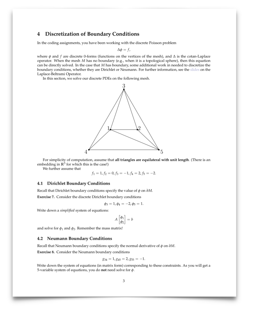
Warning: The original version of this assignment had an unsolvable linear system in Exercise 7. I updated the assignment on Thursday, so hopefully the exercise is possible now.

Assignment 5 [Coding]: Geodesic Distance (Due 5/2)

For the coding portion of this assignment, you will implement the heat method, which is an algorithm for computing geodesic distance on curved surfaces. All of the details you need for implementation are described in Section 3 of the paper, up through and including Section 3.2. Note that you need only be concerned with the case of triangle meshes (not polygon meshes or point clouds); pay close attention to the paragraph labeled “Choice of Timestep.”

Please implement the following routines in:

  1. projects/geodesic-distances/heat-method.js:
    1. constructor
    2. computeVectorField
    3. computeDivergence
    4. compute

Notes

  • Refer to sections 3.2 of the paper for discretizations of Algorithm 1 (page 3).
  • Recall that our Laplace matrix is positive semidefinite, which might differ from the sign convention the authors use.
  • The tests for computeVectorField and computeDivergence depend on the A and F matrices you define in your constructor. So if you fail the tests but your functions look correct, check whether you have defined the flow and laplace matrices properly.
  • Your solution should implement zero neumann boundary conditions (which are the “default behavior” of the cotan Laplacian) but feel free to tryout other Dirichlet and Neumann boundary conditions on your own.

Submission Instructions

Please rename your heat-method.js file to heat-method.txt and put it in a single zip file called solution.zip. This file and your solution to the written exercises should be submitted together in a single email to Geometry.Collective@gmail.com with the subject line DDG19A4.

Assignment 4 [Written]: Conformal Parameterization (Due 4/16)


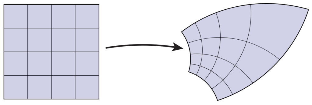
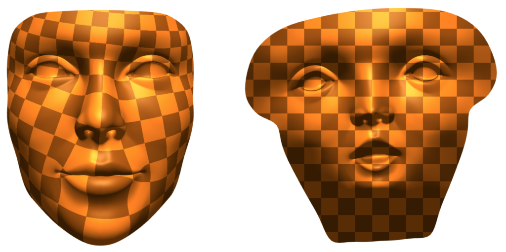
The written part of your next assignment, on conformal surface flattening, is now available below. Conformal flattening is important for (among other things) making the connection between processing of 3D surfaces, and existing fast algorithms for 2D image processing. You’ll have the opportunity to implement one of these algorithms in the coding part of the assignment.


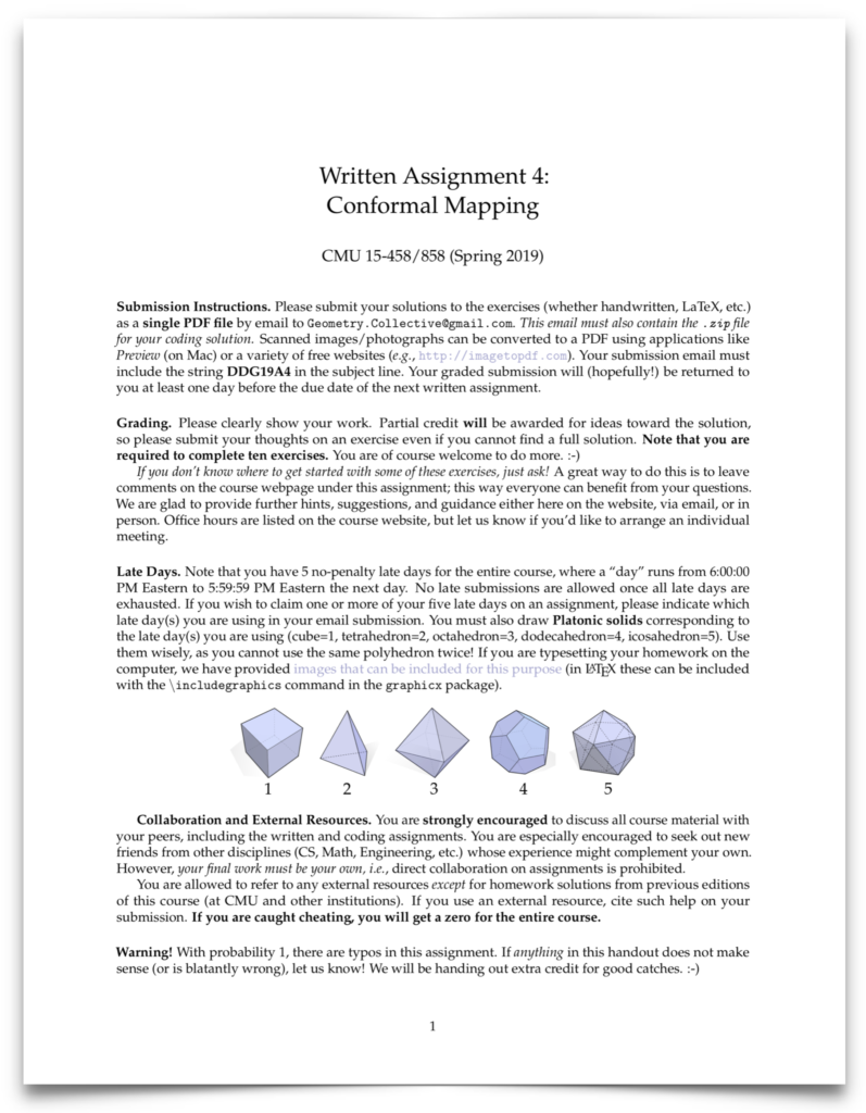
Assignment 4

Assignment 4 [Coding]: Conformal Parameterization (Due 4/16)

For the coding portion of your assignment on conformal parameterization, you will implement the Spectral Conformal Parameterization (SCP) algorithm as described in the course notes.Please implement the following routines in

  1. core/geometry.js:
    1. complexLaplaceMatrix
  2. projects/parameterization/spectral-conformal-parameterization.js:
    1. buildConformalEnergy
    2. flatten
  3. utils/solvers.js:
    1. solveInversePowerMethod
    2. residual

Notes

  • I added a few tests for utils/solvers.js. They’re available in the git repository. If you’re familiar with git, you can pull the changes. If you’d prefer not to mess around with git, you can also just download the files and put them in tests/utils.
    • Warning: I fixed a problem with the residual test. In the notes, the residual is defined as a vector $Ax – \lambda x$. But your function residual should return a float. You should return $\frac{\|Ax – \lambda x\|_2}{\|x\|_2}$. Furthermore, you should compute $\lambda$ as $\frac{x^\dagger A x}{x^\dagger x}$ where $x^\dagger$ is the conjugate transpose of $x$.
  • The complex version of the cotan-Laplace matrix can be built in exactly the same manner as its real counterpart. The only difference now is that the cotan values of our matrix will be complex numbers with a zero imaginary component. This time, we will work with meshes with boundary, so your Laplace matrix will have to handle boundaries properly (you just have to make sure your cotan function returns 0 for halfedges which are in the boundary).
  • The buildConformalEnergy function builds a $|V| \times |V|$ complex matrix corresponding to the conformal energy $E_C(z) = E_D(z) – \mathcal A(Z)$ where $E_D$ is the Dirichlet energy (given by our complex cotan-Laplace matrix) and $\mathcal A$ is the total signed area of the region $z(M)$ in the complex plane (Please refer to Section 7.4 of the notes for more details). You may find it easiest to iterate over the halfedges of the mesh boundaries to construct the area matrix (Recall that the Mesh object has a boundaries variable which stores all the boundary loops.
  • The flatten function returns a dictionary mapping each vertex to a vector (linear-algebra/vector.js) of planar coordinates by finding the eigenvector corresponding to the smallest eigenvalue of the conformal energy matrix. You can compute this eigenvector by using solveInversePowerMethod (described below).
  • Your solveInversePowerMethod function should implement Algorithm 1 in Section 7.5 of the course notes with one modification – after computing $Ay_i = y_{i-1}$, center $y_i$ around the origin by subtracting its mean. You don’t have to worry about the $B$ matrix or generalized eigenvalue problem. Important: Terminate your iterations when your residual is smaller that 10^-10.
  • The parameterization project directory also contains a basic implementation of the Boundary First Flattening (BFF) algorithm. Feel free to play around with it in the viewer and compare the results to your SCP implementation.

Submission Instructions

Please rename your geometry.js, spectral-conformal-parameterization.js and solvers.js files to geometry.txt, spectral-conformal-parameterization.txt and solvers.txt (respectively) and put them in a single zip file called solution.zip. These files and your solution to the written exercises should be submitted together in a single email to Geometry.Collective@gmail.com with the subject line DDG19A4.

Assignment 3 [Coding]: The Laplacian (Due 4/2)

For the coding portion of this assignment, you will build the so-called “cotan-Laplace” matrix and start to see how it can be used for a broad range of surface processing tasks, including the Poisson equation and two kinds of curvature flow.


Getting Started

Please implement the following routines in

  1. core/geometry.js:
    • laplaceMatrix
    • massMatrix
  2. projects/poisson-problem/scalar-poisson-problem.js:
    • constructor
    • solve
  3. projects/geometric-flow/mean-curvature-flow.js:
    • buildFlowOperator
    • integrate
  4. projects/geometric-flow/modified-mean-curvature-flow.js:
    • constructor
    • buildFlowOperator


Notes

  • Sections 6.4-6 of the course notes describe how to build the cotan-Laplace matrix and mass matrices, and outline how they can be used to solve equations on a mesh. In these applications you will be required to setup and solve a linear system of equations $Ax=b$ where $A$ is the Laplace matrix, or some slight modification thereof. Highly efficient numerical methods such as Cholesky Factorization can be used to solve such systems, but require A to be symmetric positive definite. Notice that the cotan-Laplace matrix described in the notes is negative semi-definite. To make it compatible for use with numerical methods like the Cholesky Factorization, your implementation of laplaceMatrix should instead produce a positive definite matrix, i.e., it should represent the expression
    $$(\Delta u)_i=\frac12 \sum_{ij}(\cot \alpha_{ij}+\cot \beta_{ij})(u_i–u_j).$$(Note that $u_i−u_j$ is reversed relative to the course notes.) To make this matrix strictly positive definite (rather than semidefinite), you should also add a small offset such as $10^{-8}$ to the diagonal of the matrix (which can be expressed in code as a floating point value 1e-8). This technique is known as Tikhonov regularization.
  • The mass matrix is a diagonal matrix containing the barycentric dual area of each vertex.
  • In the scalar Poisson problem, your goal is to discretize and solve the equation $\Delta \phi = \rho$ where $rho$ is a scalar density on vertices and $\Delta$ is the Laplace operator. Be careful about appropriately incorporating dual areas into the discretization of this equation (i.e., think about where and how the mass matrix should appear); also remember that the right-hand side cannot have a constant component (since then there is no solution).
  • In your implementation of the implicit mean curvature flow algorithm, you can encode the surface $f:M \to \mathbb R^3$ as a single DenseMatrix of size $|V| \times 3$, and solve with the same (scalar) cotan-Laplace matrix used for the previous part. When constructing the flow operator, you should follow section 6.6 of the notes. But be careful – when we discretize equations of the form $\Delta f = \rho$, we create systems of the form $A f = M \rho$. So you’ll need to add in the mass matrix somewhere. Also, recall that our discrete Laplace matrix is the negative of the actual Laplacian.
  • The modified mean curvature flow is nearly identical to standard mean curvature flow. The one and only difference is that you should not update the cotan-Laplace matrix each time step, i.e., you should always be using the cotans from the original input mesh. The mass matrix, however, must change on each iteration.


Submission Instructions

Please rename your geometry.js, scalar-poisson-problem.js, mean-curvature-flow.js and modified-mean-curvature-flow.js files to geometry.txt, scalar-poisson-problem.txt, mean-curvature-flow.txt and modified-mean-curvature-flow.txt (respectively) and put them in a single zip file called solution.zip. These files and your solution to the written exercises should be submitted together in a single email to Geometry.Collective@gmail.com with the subject line DDG19A3.

Assignment 3 [Written]: The Laplacian (Due 4/2)

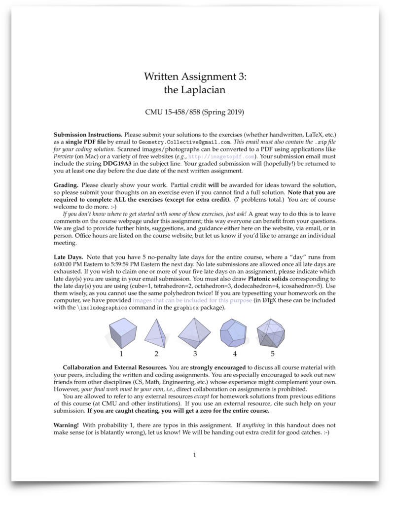
These exercises will lead you through two different derivations for the cotan-Laplace operator. As we’ll discuss in class, this operator is basically the “Swiss army knife” of discrete differential geometry and digital geometry processing, opening the door to a huge number of interesting algorithms and applications. Note that this time the exercises all come from the course notes—you will need to read the accompanying notes in order to familiarize yourself with the necessary material (though actually we’ve covered much of this stuff in class already!)


Assignment 2 (Written): Investigating Curvature (Due 3/19)

The written portion of Assignment 2 can be found below. It takes a look at the curvature of smooth and discrete surfaces, which we have been talking about in lecture. Note that you are required to complete only two problems from each section!

Warning: We renumbered the Exercises in the course notes to make more sense, so you make sure you refer to the updated notes when doing these exercises.

Assignment 2 (Coding): Investigating Curvature (Due 3/19)


For the coding portion of this assignment, you will implement various expressions for discrete curvatures and surfaces normals that you will derive in the written assignment. (However, the final expressions are given below in case you want to do the coding first.) Once implemented, you will be able to visualize these geometric quantities on a mesh. For simplicity, you may assume that the mesh has no boundary.


Getting Started
Please implement the following routines in core/geometry.js:

  1. angle
  2. dihedralAngle
  3. vertexNormalAngleWeighted
  4. vertexNormalSphereInscribed
  5. vertexNormalAreaWeighted
  6. vertexNormalGaussianCurvature
  7. vertexNormalMeanCurvature
  8. angleDefect
  9. totalAngleDefect
  10. scalarMeanCurvature
  11. circumcentricDualArea
  12. principalCurvatures


Notes 

1. The dihedral angle between the normals $N_{ijk}$ and $N_{ijl}$ of two adjacent faces $ijk$ and $ijl$ (respectively) is given by
$$ \theta_{ij} := \text{atan2}\left(\frac{e_{ij}}{\|e_{ij}\|} \cdot \left(N_{ijk} \times N_{jil}\right), N_{ijk} \cdot N_{jil}\right)$$

where $e_{ij}$ is the vector from vertex $i$ to vertex $j$.

2. The formulas for the angle weighted normal, sphere inscribed normal, area weighted normal, discrete Gaussian curvature normal and discrete mean curvature normal at vertex $i$ are
\[\begin{aligned}
N_i^\phi &:= \sum_{ijk \in F} \phi_i^{jk}N_{ijk}\\
N_i^S &:= \sum_{ijk \in F} \frac{e_{ij} \times e_{ik}} {\|e_{ij}\|^2\|e_{ik}\|^2}\\
N_i^A &:= \sum_{ijk \in F} A_{ijk}N_{ijk}\\
KN_i &= \frac 12 \sum_{ij \in E} \frac{\theta_{ij}}{\|e_{ij}\|}e_{ij}\\
HN_i &= \frac 12 \sum_{ij \in E}\left(\cot\left(\alpha_k^{ij}\right) + \cot\left(\beta_l^{ij}\right)\right)e_{ij}
\end{aligned}
\]

where $\phi_i^{jk}$ is the interior angle between edges $e_{ij}$ and $e_{ik}$, and $A_{ijk}$ is the area of face $ijk$. Note that sums are taken only over elements (edges or faces) containing vertex $i$. Normalize the final value of all your normal vectors before returning them.

3. The circumcentric dual area at vertex $i$ is given by
\[A_i := \frac 18 \sum_{ijk \in F} \|e_{ik}\|^2\cot\left(\alpha_j^{ki}\right) + \|e_{ij}\|^2\cot\left(\beta_k^{ij}\right)\]

4. The discrete scalar Gaussian curvature (also known as angle defect) and discrete scalar mean curvature at vertex $i$ are given by
\[\begin{aligned}
K_i &:= 2\pi – \sum_{ijk \in F} \phi_i^{jk}\\
H_i &:= \frac 12 \sum_{ij \in E} \theta_{ij}\|e_{ij}\|
\end{aligned}
\]

Note that these quantities are discrete 2-forms, i.e., they represent the total Gaussian and mean curvature integrated over a neighborhood of a vertex. They can be converted to pointwise quantities (i.e., discrete 0-forms at vertices) by dividing them by the  circumcentric dual area of the vertex (i.e., by applying the discrete Hodge star).

5. You are required to derive expressions for the principal curvatures $\kappa_1$ and $\kappa_2$ in exercise 4 of the written assignment. Your implementation of principalCurvatures should return the (pointwise) minimum and maximum principal curvature values at a vertex (in that order).

Submission Instructions

Please rename your geometry.js file to geometry.txt and put it in a single zip file called solution.zip. This file and your solution to the written exercises should be submitted together in a single email to Geometry.Collective@gmail.com with the subject line DDG19A2.