Lecture 11: Discrete Curves

This lecture presents the discrete counterpart of the previous lecture on smooth curves. Here we arrive at a discrete version of the fundamental theorem for plane curves: a discrete curve is completely determined by its discrete parameterization (a.k.a. edge lengths) and its discrete curvature (a.k.a. exterior angles). We’ll also cook up a discrete version of the fundamental theorem for space curves, and give a bunch of neat examples of discrete curves in geometry processing and physical simulation.

Assignment 2 (Coding): Investigating Curvature (due 3/25)


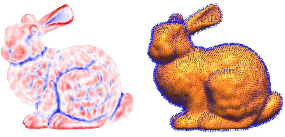
For the coding portion of this assignment, you will implement various expressions for discrete curvatures and surfaces normals that you will derive in the written assignment. (However, the final expressions are given below in case you want to do the coding first.) Once implemented, you will be able to visualize these geometric quantities on a mesh. For simplicity, you may assume that the mesh has no boundary.


Getting Started
Please implement the following routines in core/geometry.[js|cpp]:

  1. angle
  2. dihedralAngle
  3. vertexNormalAngleWeighted
  4. vertexNormalSphereInscribed
  5. vertexNormalAreaWeighted
  6. vertexNormalGaussianCurvature
  7. vertexNormalMeanCurvature
  8. angleDefect
  9. totalAngleDefect
  10. scalarMeanCurvature
  11. circumcentricDualArea
  12. principalCurvatures


Notes 

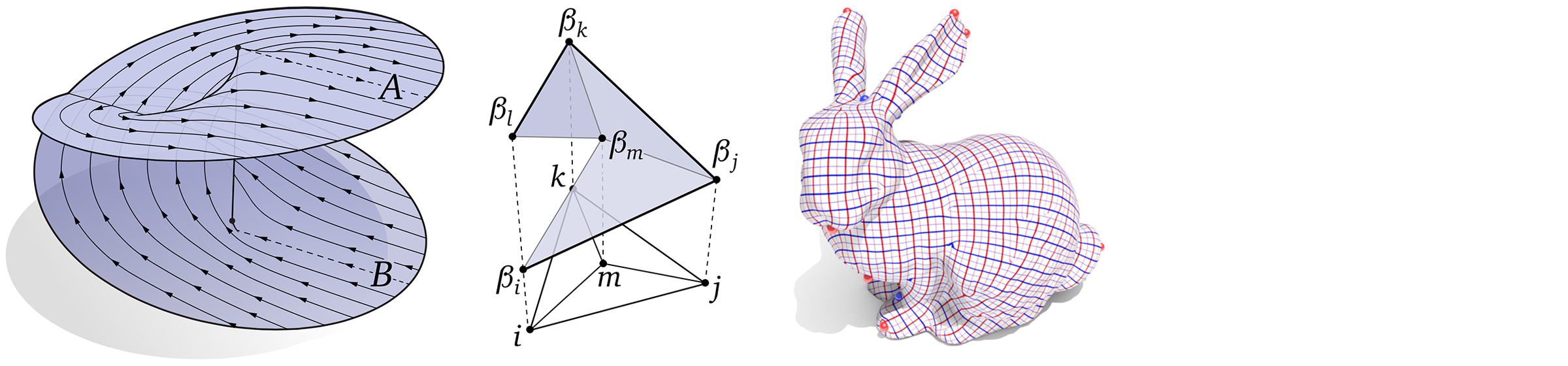
1. The dihedral angle between the normals $N_{ijk}$ and $N_{ijl}$ of two adjacent faces $ijk$ and $ijl$ (respectively) is given by
$$ \theta_{ij} := \text{atan2}\left(\frac{e_{ij}}{\|e_{ij}\|} \cdot \left(N_{ijk} \times N_{jil}\right), N_{ijk} \cdot N_{jil}\right)$$

where $e_{ij}$ is the vector from vertex $i$ to vertex $j$.

2. The formulas for the angle weighted normal, sphere inscribed normal, area weighted normal, discrete Gaussian curvature normal and discrete mean curvature normal at vertex $i$ are
\[\begin{aligned}
N_i^\phi &:= \sum_{ijk \in F} \phi_i^{jk}N_{ijk}\\
N_i^S &:= \sum_{ijk \in F} \frac{e_{ij} \times e_{ik}} {\|e_{ij}\|^2\|e_{ik}\|^2}\\
N_i^A &:= \sum_{ijk \in F} A_{ijk}N_{ijk}\\
KN_i &= \frac 12 \sum_{ij \in E} \frac{\theta_{ij}}{\|e_{ij}\|}e_{ij}\\
HN_i &= \frac 12 \sum_{ij \in E}\left(\cot\left(\alpha_k^{ij}\right) + \cot\left(\beta_l^{ij}\right)\right)e_{ij}
\end{aligned}
\]

where $\phi_i^{jk}$ is the interior angle between edges $e_{ij}$ and $e_{ik}$, and $A_{ijk}$ is the area of face $ijk$. Note that sums are taken only over elements (edges or faces) containing vertex $i$. Normalize the final value of all your normal vectors before returning them.

3. The circumcentric dual area at vertex $i$ is given by
\[A_i := \frac 18 \sum_{ijk \in F} \|e_{ik}\|^2\cot\left(\alpha_j^{ki}\right) + \|e_{ij}\|^2\cot\left(\beta_k^{ij}\right)\]

4. The discrete scalar Gaussian curvature (also known as angle defect) and discrete scalar mean curvature at vertex $i$ are given by
\[\begin{aligned}
K_i &:= 2\pi – \sum_{ijk \in F} \phi_i^{jk}\\
H_i &:= \frac 12 \sum_{ij \in E} \theta_{ij}\|e_{ij}\|
\end{aligned}
\]

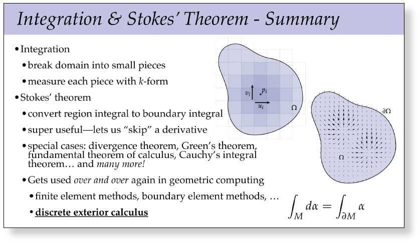
Note that these quantities are discrete 2-forms, i.e., they represent the total Gaussian and mean curvature integrated over a neighborhood of a vertex. They can be converted to pointwise quantities (i.e., discrete 0-forms at vertices) by dividing them by the  circumcentric dual area of the vertex (i.e., by applying the discrete Hodge star).

5. You are required to derive expressions for the principal curvatures $\kappa_1$ and $\kappa_2$ in exercise 4 of the written assignment. Your implementation of principalCurvatures should return the (pointwise) minimum and maximum principal curvature values at a vertex (in that order).

Submission Instructions

Please submit only the source code file geometry.js or geometry.cpp (depending on whether you’re using JavaScript or C++). This means your code should not depend on edits made to any other files. Then follow the usual hand-in instructions.

The assignment is due on March 25, 2022 at 5:59:59pm Eastern (not at midnight!).

Note that we are giving you more time to do this assignment than other ones, since we know you have midterms in other classes! 🙂

Assignment 2 (Written): Investigating Curvature (due 3/25)

The written portion of Assignment 2 can be found below. It takes a look at the curvature of smooth and discrete surfaces, which we have been talking about in lecture.

If you’re typesetting this assignment, feel free to use this template.

The assignment is due on March 25, 2022 at 5:59:59pm Eastern (not at midnight!).

Note that we are giving you more time to do this assignment than other ones, since we know you have midterms in other classes! 🙂

Lecture 10: Smooth Curves

After spending a great deal of time understanding some basic algebraic and analytic tools (exterior algebra and exterior calculus), we’ll finally start talking about geometry in earnest, starting with smooth plane and space curves. Even low-dimensional geometry like curves reveal a lot of the phenomena that arise when studying curved manifolds in general. Our main result for this lecture is the fundamental theorem of space curves, which reveals that (loosely speaking) a curve is entirely determined by its curvatures. Descriptions of geometry in terms of “auxiliary” quantities such as curvature play an important role in computation, since different algorithms may be easier or harder to formulate depending on the quantities or variables used to represent the geometry. Next lecture, for instance, we’ll see some examples of algorithms for curvature flow, which naturally play well with representations based on curvature!

Reading 5—Curves and Surfaces (due 3/15)

Your next reading complements our in-class discussion of the geometry of curves and surfaces. In particular, you should read Chapter 3 of the course notes, pages 28–44. This reading is due next Wednesday, March 31.

Handin instructions are described on the Assignments Page.

Since these notes just barely scratch the surface (literally), I am often asked for recommendations on books that provide a deeper discussion of surfaces. The honest answer is, “I don’t know; I mostly didn’t learn it from a book.” But there are a couple fairly standard references (other) people seem to like, both of which should be available digitally from the CMU library:

Your short 2-3 sentence summary is due by 10am Eastern on March 15, 2022.  Handin instructions can be found on the assignment page.

Supplemental: Vector-Valued Differential Forms

This short-but-important supplemental lecture introduces some language we’ll need for describing geometry (curves, surfaces, etc.) in terms of differential forms. So far, we’ve said that a differential \(k\)-form produces a scalar measurement. But when talking about geometry, we often care about quantities that are vector-valued rather than scalar-valued. For instance, positions in \(\mathbb{R}^n\), tangents, and normals are all vector-valued quantities. For the most part, all of our operations look pretty much the same as before. The one exception is the wedge product, which in \(\mathbb{R}^3\) we now define in terms of the cross product.

Lecture 9: Discrete Exterior Calculus

This lecture wraps up our discussion of discrete exterior calculus, which will provide the basis for many of the algorithms we’ll develop in this class. Here we’ll encounter the same operations as in the smooth setting (Hodge star, wedge product, exterior derivative, etc.), which in the discrete setting are encoded by simple matrices that translate problems involving differential forms into ordinary linear algebra problems.

Lecture 8: Discrete Differential Forms

In this lecture, we turn smooth differential \(k\)-forms into discrete objects that we can actually compute with. The basic idea is actually quite simple: to capture some information about a differential \(k\)-form, we integrate it over each oriented \(k\)-simplex of a mesh. The resulting values are just ordinary numbers that give us some sense of what the original \(k\)-form must have looked like.

Lecture 7: Integration

Our first lecture on exterior calculus covered differentiation; our second lecture completes the picture by discussing integration of differential forms. The relationship between integration and differentiation is encapsulated by Stokes’ theorem, which generalizes the fundamental theorem of calculus, as well as many other important theorems from vector calculus and complex analysis (divergence theorem, Green’s theorem, Cauchy’s integral formula, etc.). Stokes’ theorem also plays a key role in numerical discretization of geometric problems, appearing for instance in finite volume methods and boundary element methods; for us it will be the essential tool for developing a discrete version of differential forms that we can actually compute with.

  • Video
  • Slides
  • Lecture 6: Exterior Derivative

    Ordinary calculus provides tools for understanding rates of change (via derivatives), total quantities (via integration), and the total change (via the fundamental theorem of calculus). Exterior calculus generalizes these ideas to \(n\)-dimensional quantities that arise throughout geometry and physics. Our first lecture on exterior calculus studies the exterior derivative, which describes the rate of change of a differential form, and (together with the Hodge star) generalizes the gradient, divergence, and curl operators from standard vector calculus.