Lectures 21 & 22 — Geodesics

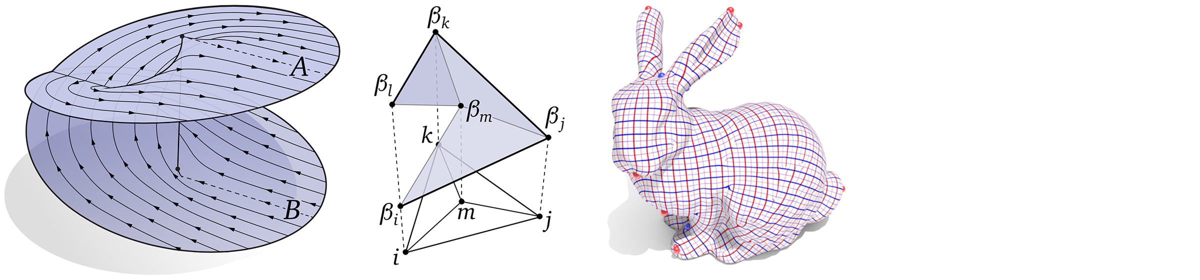
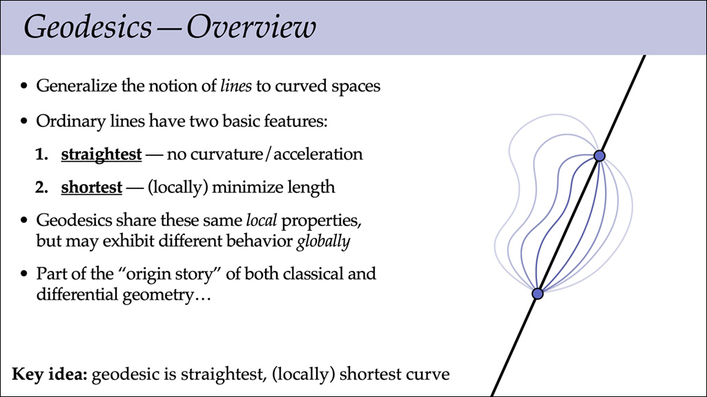
Our final lectures for the term focus on geodesics, which generalize the notion of “straight line” to curved spaces; this material also connects to your final assignment, on computing geodesic distance. Once again we’ll play “The Game” of discrete differential geometry, and see how two natural characterizations from the smooth setting (straightest and locally shortest) lead to two distinct, and fascinating definitions in the discrete setting. Along the way we’ll also encounter many rich topics from (discrete) differential geometry including the cut locus, the medial axis, the exponential/log map, the covariant derivative, and the Lie bracket! We’ll also see how all this stuff connects with practical algorithms for things like surface reconstruction from points, and give two different algorithms for tracing out geodesics on curved surfaces.

Note that the lecture video comprises about two lectures (about two hours total). If you need to watch the video instead of attending lecture (e.g., because you’re sick), we’d recommend watching it in two logical chunks:

  • Part I: Shortest Geodesics – 0:00—1:04
  • Part II: Straightest Geodesics – 1:04–1:55

Lecture 19: Conformal Geometry

A basic task in geometric algorithms is finding mappings between surfaces, which can be used to transfer data from one place to another. A particularly nice class of mappings (both from a mathematical and computational perspective) are conformal maps, which preserve angles between vectors, and are generally very well-behaved. In this first lecture we’ll take a look at smooth characterizations of conformal maps, which will ultimately inspire the way we talk about conformal maps in the discrete/computational setting.

The video covering both today and Thursday’s lecture (on discrete aspects of conformal maps) can be found here.

Lecture 18: The Laplace-Beltrami Operator

In this lecture we take a close look at the Laplacian, and its generalization to curved spaces via the Laplace-Beltrami operator. The Laplacian is one of the most fundamental objects in geometry and physics, and which plays a major role in algorithms. Here we consider several perspectives to build up some basic intuition about what the Laplacian is, and what it means.

Lecture 16—Discrete Curvature I (Integral Viewpoint)

Just as curvature provides powerful ways to describe and analyze smooth surfaces, discrete curvatures provide a powerful way to encode and manipulate digital geometry—and is a fundamental component of many modern algorithms for surface processing. This first of two lectures on discrete curvature from the integral viewpoint, i.e., integrating smooth expressions for discrete curvatures in order to obtain curvature formulae suitable for discrete surfaces. In the next lecture, we will see a complementary variational viewpoint, where discrete curvatures arise by instead taking derivatives of discrete geometry. Amazingly enough, these two perspectives will fit together naturally into a unified picture that connects essentially all of the standard discrete curvatures for triangle meshes.

Lecture 15: Curvature of Surfaces

Much of the geometry we encounter in everyday life (such as curves and surfaces sitting in space) is well-described by it curvatures. For instance, the fundamental theorem for plane curves says that an arc-length parameterized plane curve is determined by its curvature function, up to rigid motions. Similar statements can be made about surfaces and their curvatures, which we explore in this lecture.

Lecture 14: Discrete Surfaces

Discrete Surfaces

We’ll follow up our lecture on smooth surfaces with a view of surfaces from the discrete point of view. Our goal will be to translate basic concepts (such as the differential, immersions, etc.) into a purely discrete language. Here we’ll also start to see the benefit of developing discrete differential forms: many of the statements we made about surfaces in the smooth setting can be translated into the discrete setting with minimal effort. As we move forward with discrete differential geometry, this “easy translation” will enable us to take advantage of deep insights from differential geometry to develop practical computational algorithms.

Lecture 12: Smooth Surfaces I

This lecture takes a first look at smooth surfaces. There’s of course way more to know about surfaces than we can pack into a single lecture (and we’ll see plenty more later on), but this lecture will cover two very important perspectives: the extrinsic description of a surface via a local parameterization, which tells us where points sit in space, and the intrinsic description of a surface via coordinate charts, which lets us work with a surface without worrying how it’s embedded in space.

Lecture 11: Discrete Curves

This lecture presents the discrete counterpart of the previous lecture on smooth curves. Here we arrive at a discrete version of the fundamental theorem for plane curves: a discrete curve is completely determined by its discrete parameterization (a.k.a. edge lengths) and its discrete curvature (a.k.a. exterior angles). We’ll also cook up a discrete version of the fundamental theorem for space curves, and give a bunch of neat examples of discrete curves in geometry processing and physical simulation.

Lecture 10: Smooth Curves

After spending a great deal of time understanding some basic algebraic and analytic tools (exterior algebra and exterior calculus), we’ll finally start talking about geometry in earnest, starting with smooth plane and space curves. Even low-dimensional geometry like curves reveal a lot of the phenomena that arise when studying curved manifolds in general. Our main result for this lecture is the fundamental theorem of space curves, which reveals that (loosely speaking) a curve is entirely determined by its curvatures. Descriptions of geometry in terms of “auxiliary” quantities such as curvature play an important role in computation, since different algorithms may be easier or harder to formulate depending on the quantities or variables used to represent the geometry. Next lecture, for instance, we’ll see some examples of algorithms for curvature flow, which naturally play well with representations based on curvature!