The written portion of this assignment can be found here. This time, we’re taking off the “training wheels” and having you read a real paper, rather than course notes. Why? Because you’re ready for it! At this point you have all the fundamental knowledge you need to go out into the broader literature and start implementing all sorts of algorithms that are built on top of ideas from differential geometry. In fact, this particular algorithm is not much of a departure from things you’ve done already: solving simple equations involving the Laplacian on triangle meshes. As discussed in our lecture on the Laplacian, you’ll find many algorithms in digital geometry processing that have this flavor: compute some basic data (e.g., using a local formula at each vertex), solve a Laplace-like equation, compute some more basic data, and so on. Your main references for this assignment will be:

• this video, which gives a brief (18-minute) overview of the algorithm, and
• this paper, which explains the algorithm in detail.

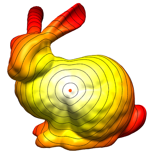
For the coding portion of this assignment, you will implement the heat method, which is an algorithm for computing geodesic distance on curved surfaces. All of the details you need for implementation are described in Section 3 of the paper, up through and including Section 3.2. Note that you need only be concerned with the case of triangle meshes (not polygon meshes or point clouds); pay close attention to the paragraph labeled “Choice of Timestep.” Please implement the following routines in:

• projects/geodesic-distances/heat-method.[js/cpp]:
  • constructor
  • computeVectorField
  • computeDivergence
  • compute

Notes

• Refer to sections 3.2 of the paper for discretizations in Algorithm 1 (page 3).
• Recall that our Laplace matrix is positive semidefinite, which might differ from the sign convention the authors use.
• The tests for computeVectorField and computeDivergence depend on the A and F matrices you define in your constructor. So if you fail the tests but your functions look correct, check whether you have defined the flow and laplace matrices properly.
• Your solution should implement zero Neumann boundary conditions (which are the “default behavior” of the cotan Laplacian) but feel free to tryout other Dirichlet and Neumann boundary conditions on your own.

Handin instructions can be found in the Assignments section of the main page.