Administrivia

On the last assignment, please be sure to use exactly the string DDG19A6 as the subject line – I don’t want to miss any of your submissions so soon before the grading deadline.

I missed a few submissions of earlier assignments due to people using a different subject – I think I’ve found all of the submissions, but it’s entirely possible that I’m still missing some. As far as I know, I have finished grading assignments 0-4. If you submitted any of those assignments but haven’t received a grade, please let me know. If you need to get in touch with me, it will probably be easier for you to email me at mgillesp@andrew.cmu.edu. The DDG class email inbox is always full of assignments/readings, so it’s easy for me to miss things.

Assignment 3 [Coding]: The Laplacian (Due 4/2)

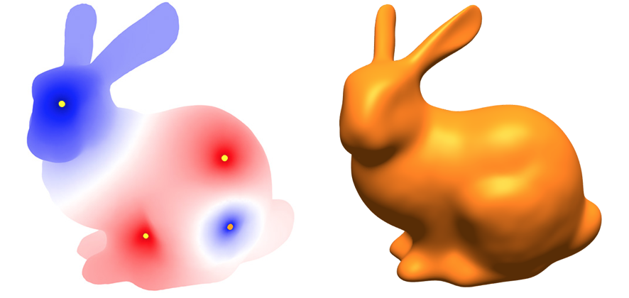
For the coding portion of this assignment, you will build the so-called “cotan-Laplace” matrix and start to see how it can be used for a broad range of surface processing tasks, including the Poisson equation and two kinds of curvature flow.


Getting Started

Please implement the following routines in

  1. core/geometry.js:
    • laplaceMatrix
    • massMatrix
  2. projects/poisson-problem/scalar-poisson-problem.js:
    • constructor
    • solve
  3. projects/geometric-flow/mean-curvature-flow.js:
    • buildFlowOperator
    • integrate
  4. projects/geometric-flow/modified-mean-curvature-flow.js:
    • constructor
    • buildFlowOperator


Notes

  • Sections 6.4-6 of the course notes describe how to build the cotan-Laplace matrix and mass matrices, and outline how they can be used to solve equations on a mesh. In these applications you will be required to setup and solve a linear system of equations $Ax=b$ where $A$ is the Laplace matrix, or some slight modification thereof. Highly efficient numerical methods such as Cholesky Factorization can be used to solve such systems, but require A to be symmetric positive definite. Notice that the cotan-Laplace matrix described in the notes is negative semi-definite. To make it compatible for use with numerical methods like the Cholesky Factorization, your implementation of laplaceMatrix should instead produce a positive definite matrix, i.e., it should represent the expression
    $$(\Delta u)_i=\frac12 \sum_{ij}(\cot \alpha_{ij}+\cot \beta_{ij})(u_i–u_j).$$(Note that $u_i−u_j$ is reversed relative to the course notes.) To make this matrix strictly positive definite (rather than semidefinite), you should also add a small offset such as $10^{-8}$ to the diagonal of the matrix (which can be expressed in code as a floating point value 1e-8). This technique is known as Tikhonov regularization.
  • The mass matrix is a diagonal matrix containing the barycentric dual area of each vertex.
  • In the scalar Poisson problem, your goal is to discretize and solve the equation $\Delta \phi = \rho$ where $rho$ is a scalar density on vertices and $\Delta$ is the Laplace operator. Be careful about appropriately incorporating dual areas into the discretization of this equation (i.e., think about where and how the mass matrix should appear); also remember that the right-hand side cannot have a constant component (since then there is no solution).
  • In your implementation of the implicit mean curvature flow algorithm, you can encode the surface $f:M \to \mathbb R^3$ as a single DenseMatrix of size $|V| \times 3$, and solve with the same (scalar) cotan-Laplace matrix used for the previous part. When constructing the flow operator, you should follow section 6.6 of the notes. But be careful – when we discretize equations of the form $\Delta f = \rho$, we create systems of the form $A f = M \rho$. So you’ll need to add in the mass matrix somewhere. Also, recall that our discrete Laplace matrix is the negative of the actual Laplacian.
  • The modified mean curvature flow is nearly identical to standard mean curvature flow. The one and only difference is that you should not update the cotan-Laplace matrix each time step, i.e., you should always be using the cotans from the original input mesh. The mass matrix, however, must change on each iteration.


Submission Instructions

Please rename your geometry.js, scalar-poisson-problem.js, mean-curvature-flow.js and modified-mean-curvature-flow.js files to geometry.txt, scalar-poisson-problem.txt, mean-curvature-flow.txt and modified-mean-curvature-flow.txt (respectively) and put them in a single zip file called solution.zip. These files and your solution to the written exercises should be submitted together in a single email to Geometry.Collective@gmail.com with the subject line DDG19A3.

Steiner Formula for Surfaces in \(\mathbb{R}^3\)

In the slides we derived a Steiner formula for polyhedral surfaces in \(\mathbb{R}^3\), by considering the Minkowski sum with a ball and working out expressions for the areas and curvatures associated with vertices, edges, and faces. But we can also get a Steiner formula for smooth surfaces, using the expressions already derived in class. In particular, recall that for a closed surface \(f: M \to \mathbb{R}^3\) with Gauss map \(N\), we can obtain the basic curvatures by just wedging together \(df\) and \(dN\) in all possible ways:
\[\begin{array}{rcl}
df \wedge df &=& 2NdA \\
df \wedge dN &=& 2HNdA \\
dN \wedge dN &=& 2KNdA \\
\end{array}
\]
Here \(H\) and \(K\) denote the mean and Gauss curvature (resp.), and dA is the area form induced by \(f\). For sufficiently small \(t\), taking a Minkowski sum with a ball is the same as pushing the surface in the normal direction a distance \(t\). In other words, the surface
\[
f_t := f + tN
\]
will describe the “outer” boundary of the Minkowski sum; this surface has the same Gauss map \(N\) as the original one. To get its area element, we can take the wedge product
\[
\begin{array}{rcl}
df_t \wedge df_t
&=& (df + t dN) \wedge (df + t dN) \\
&=& df \wedge df + 2t df \wedge dN + t^2 dN \wedge dN,
\end{array}
\]
where we have used the fact that \(\alpha \wedge \beta = \beta \wedge \alpha\) when \(\alpha,\beta\) are both \(\mathbb{R}^3\)-valued 1-forms. The list of identities above then yields
\[
df_t \wedge df_t = (2 + 4tH + 2t^2 K)NdA,
\]
or equivalently,
\[
\fbox{\(dA_t = (1+2tH+t^2K)dA.\)}
\]
In other words, just as in the polyhedral case, the rate at which the area is growing is a polynomial in the ball radius \(t\); the coefficients of this polynomial are given by the basic curvatures of the surface (also known as quermassintegrals!).

Assorted things about homework

  1. Here’s a piece of advice for assignment 1 which I forgot to put in the original post: You can compute the ratio of dual edge lengths to primal edge lengths using the cotan formula, which can be found on Slide 28 of the Discrete Exterior Calculus lecture, or in exercise 36 of the notes (you don’t have to do the exercise for this homework).
  2. I just emailed out grades for assignment 0. If you have questions or concerns about your graded assignment, or if you did not receive a graded assignment, please feel free to email me or to talk to me during office hours.
  3. Very few people have been attending my office hours on Fridays, so I am moving my office hours to be 2:30pm-4pm on Monday afternoons. They will still be held outside of Smith 232.
  4. If you would like to see solutions for assignment 0, we will bring some printed copies to class on Tuesday. I can also print you solutions if you stop by during office hours.

Office Hours + Homework Typo

I will hold office hours tomorrow (Friday Feb. 1) in the Smith Hall 2nd floor open space from 3pm to 4pm. Next week, since the homework is due on Thursday, I will hold office hours on Tuesday from 3pm to 4pm in the same place. After that, I will go back to having office hours on Fridays.

Sorry for the short notice. If these times don’t work for you, feel free to email me and we can arrange to meet another time.


Also, somebody pointed out a typo in the coding assignment during recitation – the vertex-edge and edge-face adjacency matrices should be sparse matrices, not dense like it says in the comments/documentation.

Assignment -1: Favorite Formula

Part of your course grade is determined by participation, which can include both in-class participation as well as discussion here on the course webpage.  Therefore, your first assignment is to:

  1. create an account, and
  2. leave a comment on this post containing your favorite mathematical formula (see below).
To make things interesting, your comment should include a description of your favorite mathematical formula typeset in $\LaTeX$.  If you don’t know how to use $\LaTeX$ this is a great opportunity to learn — a very basic introduction can be found here.  (And if you don’t have a favorite mathematical formula, this is a great time to pick one!)
 
(P.S. Anyone interested in hearing about some cool “favorite theorems” should check out this podcast.)

Welcome to Discrete Differential Geometry! (Spring 2019)

Welcome to the website for 15-458/858 (Discrete Differential Geometry).  Here you’ll find course notes, lecture slides, and homework (see links on the right).

If you are a student in the class, register now by clicking here!

To participate in the class, you must register using your Andrew (CMU) email address.

A few things to note:

  • You will be subscribed to receive email notification about new posts, comments, etc.
  • You can ask questions by leaving a comment on a post.  If you’re apprehensive about asking questions in public, feel free to register under a pseudonym.
  • Otherwise, please associate a picture to your profile by registering your email address at Gravatar.com—doing so will help us better recognize you in class!
  • You can include mathematical notation in your questions using standard $\LaTeX$ syntax.  For instance, when enclosed in a pair of dollar signs, an expression like dollar\int_M K dA = 2\pi\chidollar gets typeset as $\int_M K dA = 2\pi\chi$.
If you encounter any problems while trying to use the website, please contact the TA (listed under the course description).