Lecture 7: Integration

Our first lecture on exterior calculus covered differentiation; our second lecture completes the picture by discussing integration of differential forms. The relationship between integration and differentiation is encapsulated by Stokes’ theorem, which generalizes the fundamental theorem of calculus, as well as many other important theorems from vector calculus and complex analysis (divergence theorem, Green’s theorem, Cauchy’s integral formula, etc.). Stokes’ theorem also plays a key role in numerical discretization of geometric problems, appearing for instance in finite volume methods and boundary element methods; for us it will be the essential tool for developing a discrete version of differential forms that we can actually compute with.

  • Video
  • Slides
  • Lecture 6: Exterior Derivative

    Ordinary calculus provides tools for understanding rates of change (via derivatives), total quantities (via integration), and the total change (via the fundamental theorem of calculus). Exterior calculus generalizes these ideas to \(n\)-dimensional quantities that arise throughout geometry and physics. Our first lecture on exterior calculus studies the exterior derivative, which describes the rate of change of a differential form, and (together with the Hodge star) generalizes the gradient, divergence, and curl operators from standard vector calculus.

    Assignment 1 (Written): Exterior Calculus (Due 3/18)

    The written portion of assignment 1 is now available, which covers some of the fundamental tools we’ll be using in our class. Initially this assignment may look a bit intimidating, but the homework is not as long as it might seem: all the text in the big gray blocks contains supplementary, formal definitions that you do not need to know in order to complete the assignments.

    Don’t be shy about asking us questions here in the comments, via email, or during office hours.  We want to help you succeed on this assignment, so that you can enjoy all the adventures yet to come…
    A1Written

    This assignment is due on Thursday, March 18.

    Assignment 1 (Coding): Exterior Calculus (Due 3/18)

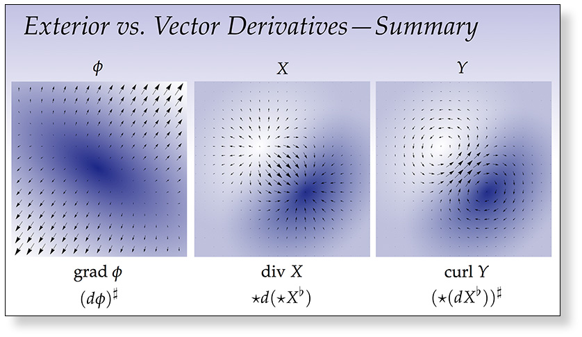
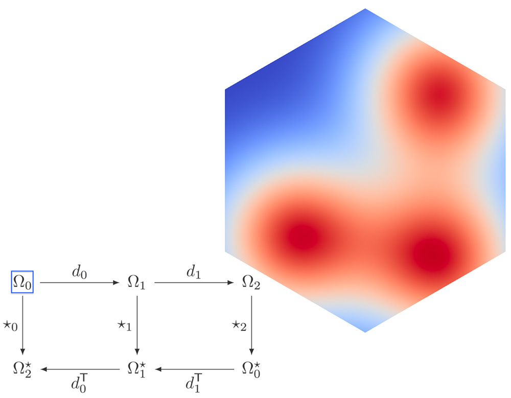
    For the coding portion of your first assignment, you will implement the discrete exterior calculus (DEC) operators $\star_0, \star_1, \star_2, d_0$ and $d_1$. Once implemented, you will be able to apply these operators to a scalar function (as depicted above) by pressing the “$\star$” and “$d$” button in the viewer. The diagram shown above will be updated to indicate what kind of differential k-form is currently displayed. These basic operations will be the starting point for many of the algorithms we will implement throughout the rest of the class; the visualization (and implementation!) should help you build further intuition about what these operators mean and how they work

    Getting Started

    • For this assignment, you need to implement the following routines:
      1. in core/geometry.[js|cpp]
        1. cotan
        2. barycentricDualArea
      2. in core/discrete-exterior-calculus.[js|cpp]
        1. buildHodgeStar0Form
        2. buildHodgeStar1Form
        3. buildHodgeStar2Form
        4. buildExteriorDerivative0Form
        5. buildExteriorDerivative1Form

    In practice, a simple and efficient way to compute the cotangent of the angle $\theta$ between two vectors $u$ and $v$ is to use the cross product and the dot product rather than calling any trigonometric functions directly; we ask that you implement your solution this way. (Hint: how are the dot and cross product of two vectors related to the cosine and sine of the angle between them?)

    In case we have not yet covered it in class, the barycentric dual area associated with a vertex $i$ is equal to one-third the area of all triangles $ijk$ touching $i$.

    EDIT: You can compute the ratio of dual edge lengths to primal edge lengths using the cotan formula, which can be found on Slide 28 of the Discrete Exterior Calculus lecture, or in exercise 36 of the notes (you don’t have to do the exercise for this homework).

    Submission Instructions

    Please submit your geometry.[js|cpp] and discrete-exterior-calculus.[js|cpp] files to Gradescope.  You should not submit any other source files (and therefore, should not edit any other source files to get your code working!).

    Reading 4: Exterior Calculus — due 3/11

    The next reading assignment will wrap up our discussion of exterior calculus, both smooth and discrete. In particular, it will explore how to differentiate and integrate \(k\)-forms, and how an important relationship between differentiation and integration (Stokes’ theorem) enables us to turn derivatives into discrete operations on meshes. In particular, the basic data we will work with in the computational setting are “integrals of derivatives,” which amount to simple scalar quantities we can associate with the vertices, edges, faces, etc. of a simplicial mesh. These tools will provide the basis for the algorithms we’ll explore throughout the rest of the semester.

    The reading is the remainder of Chapter 4 from the course notes, “A Quick and Dirty Introduction to Exterior Calculus”, Sections 4.6 through 4.8 (pages 67–83). Note that you just have to read these sections; you do not have to do the written exercises; a different set of written problems will be posted later on. The reading is due Thursday, March 11 at 10am. See the assignments page for handin instructions.