In this lecture we’ll start taking a look at geodesics, which generalize the concept of a “straight line” to curved manifolds. Here again we encounter The Game of discrete differential geometry: different characterizations of geodesics—namely, straightest vs. (locally) shortest—will lead us down a path toward different discrete analogues, and ultimately, different algorithms.
Month: April 2023
Reading 9—Choose Your Own Adventure (due 4/27)
There are way more topics and ideas in Discrete Differential Geometry than we could ever hope to cover in this course. For this final reading assignment, you can choose from one of several options that we’ll cover in the remainder of our course:
- Intrinsic Triangulations. In the next couple lectures we’ll revisit polyhedral surfaces through the powerful intrinsic perspective from differential geometry, where we no longer think about how a shape sits in space (i.e., no vertex positions) but instead only have measurements of local quantities like edge lengths and corner angles. This simple twist provides a huge amount of flexibility for computation and algorithms, since there are infinitely many ways to intrinsically triangulate the same polyhedral surface without corrupting its geometry. For this reading, you should read Sharp et al, “Geometry Processing with Intrinsic Triangulations”, pp. 1–29, plus one other chapter of your choice. Summarize what you read, and say why you chose the chapter you did.
- Repulsive Geometry. In our final lecture we’ll discuss a recent perspective on drawing/embedding/optimizing shapes using so-called repulsive energies. The basic starting point is to think about charged particles (like electrons) that try to repel each-other, often producing a nice, uniform distribution of particles. Now imagine every point of a curve or surface is charged, and let it evolve to the most “self-avoiding” configuration… some very beautiful things emerge! For this reading you should read Yu et al, “Repulsive Surfaces”, pp. 1–17. Since this is a research paper, you shouldn’t be worried about understanding 100% of the details. Rather, you should just get a general feeling for the problem motivation, the approach to the solution, and the potential applications of the method.
- Tangent Direction Fields. Related to the final assignment (A6), you can choose to read one of two surveys on methods for tangent vector field processing—which should give you some additional perspective/context for this assignment. Tangent vector fields, and more generally, symmetric n-direction fields are everywhere in physical and geometric applications, and a long-running question in DDG is: how should we represent tangent-valued data on discrete surfaces? For this reading you can read either de Goes et al, “Vector Field Processing on Triangle Meshes”, pp. 5-21, and then choose two out of three of the remaining chapters: face-based, edge-based, and vertex-based vector fields. Your writeup should compare and contrast these two choices: what are the basic pros and cons? Alternatively, you can read Vaxman et al, “Directional Field Design, Synthesis, and Processing”, pp. 1–24. Here again, your writeup should focus on the trade offs between different representations.
Assignment 5 [Written]: Geodesic Distance (Due 4/27)
Here’s the writeup for your second to last assignment. This time, we’re taking off the “training wheels” and having you read a real paper, rather than course notes. Why? Because you’re ready for it! At this point you have all the fundamental knowledge you need to go out into the broader literature and start implementing all sorts of algorithms that are built on top of ideas from differential geometry. In fact, this particular algorithm is not much of a departure from things you’ve done already: solving simple equations involving the Laplacian on triangle meshes. As discussed in our lecture on the Laplacian, you’ll find many algorithms in digital geometry processing that have this flavor: compute some basic data (e.g., using a local formula at each vertex), solve a Laplace-like equation, compute some more basic data, and so on.
Your main references for this assignment will be:
- this video, which gives a brief (18-minute) overview of the algorithm, and
- this paper, which explains the algorithm in detail.
Written exercises for this assignment are found below.

Assignment 5 [Coding]: Geodesic Distance (Due 4/27)
For the coding portion of this assignment, you will implement the heat method, which is an algorithm for computing geodesic distance on curved surfaces. All of the details you need for implementation are described in Section 3 of the paper, up through and including Section 3.2. Note that you need only be concerned with the case of triangle meshes (not polygon meshes or point clouds); pay close attention to the paragraph labeled “Choice of Timestep.”
Please implement the following routines in:
- projects/geodesic-distances/heat-method.[js/cpp]:
- constructor
- computeVectorField
- computeDivergence
- compute
Notes
- Refer to sections 3.2 of the paper for discretizations in Algorithm 1 (page 3).
- Recall that our Laplace matrix is positive semidefinite, which might differ from the sign convention the authors use.
- The tests for computeVectorField and computeDivergence depend on the A and F matrices you define in your constructor. So if you fail the tests but your functions look correct, check whether you have defined the flow and laplace matrices properly.
- Your solution should implement zero Neumann boundary conditions (which are the “default behavior” of the cotan Laplacian) but feel free to tryout other Dirichlet and Neumann boundary conditions on your own.
Submission Instructions
Please submit your source files as usual to Gradescope by 5:59pm ET..
Reading 8: Geodesic Algorithms (due April 20)
This reading complements our lecture on algorithms for computing geodesic paths with an overview of algorithms for computing geodesic distances:
- Crane, Livesu, Puppo, Qin, “A Survey of Algorithms for Geodesic Paths and Distances” (2020), pp. 1–20.
As with many of our readings, the point here is to just get a broader perspective of the material covered in lecture—you are not responsible for knowing every little detail. The algorithms discussed in Section 3 especially are well-connected to the perspective & tools we’ve been developing throughout the semester (e.g., the discrete Laplacian), and will help get you prepared for the assignment on computing geodesic distance. For this reading you should summarize the high-level ideas from the first part of the survey, and any questions you might have.
Reading 7—Discrete Conformal Geometry (Due April 11)
Your next reading will take a deep dive into conformal geometry and the many ways to discretize and compute conformal maps. This subject makes some beautiful and unexpected connections to other areas of mathematics (such as circle packings, and hyperbolic geometry), and is in some sense one of the biggest “success stories” of DDG, since there is now a complete uniformization theorem that mirrors the one on the smooth side. You’ll find out more about what this all means in the reading! The reading comes from the note, “Conformal Geometry of Simplicial Surface”:

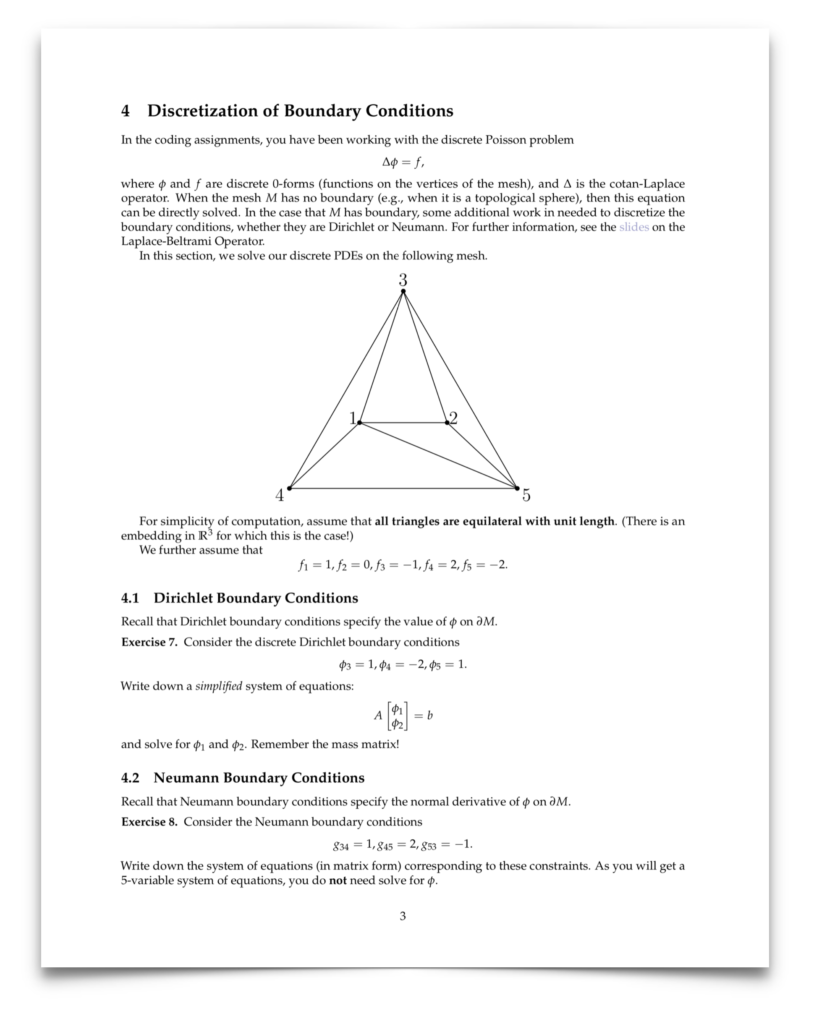
Assignment 4 [Coding]: Conformal Parameterization (Due 4/18)

For the coding portion of your assignment on conformal parameterization, you will implement the Spectral Conformal Parameterization (SCP) algorithm as described in the course notes.Please implement the following routines in
- core/geometry.[js/cpp]:
- complexLaplaceMatrix
- projects/parameterization/spectral-conformal-parameterization.[js/cpp]:
- buildConformalEnergy
- flatten
- utils/solvers.[js/cpp]:
- solveInversePowerMethod
- residual
Notes
- The complex version of the cotan-Laplace matrix can be built in exactly the same manner as its real counterpart. The only difference now is that the cotan values of our matrix will be complex numbers with a zero imaginary component. This time, we will work with meshes with boundary, so your Laplace matrix will have to handle boundaries properly (you just have to make sure your cotan function returns 0 for halfedges which are in the boundary).
- The buildConformalEnergy function builds a $|V| \times |V|$ complex matrix corresponding to the conformal energy $E_C(z) = E_D(z) – \mathcal A(Z)$ where $E_D$ is the Dirichlet energy (given by our complex cotan-Laplace matrix) and $\mathcal A$ is the total signed area of the region $z(M)$ in the complex plane (Please refer to Section 7.4 of the notes for more details). You may find it easiest to iterate over the halfedges of the mesh boundaries to construct the area matrix (Recall that the Mesh object has a boundaries variable which stores all the boundary loops.
- The flatten function returns a dictionary mapping each vertex to a vector (linear-algebra/vector.js) of planar coordinates by finding the eigenvector corresponding to the smallest eigenvalue of the conformal energy matrix. You can compute this eigenvector by using solveInversePowerMethod (described below).
- Your solveInversePowerMethod function should implement Algorithm 1 in Section 7.5 of the course notes with one modification – after computing $Ay_i = y_{i-1}$, center $y_i$ around the origin by subtracting its mean. You don’t have to worry about the $B$ matrix or generalized eigenvalue problem. Important: Terminate your iterations when your residual is smaller that 10^-10.
- The parameterization project directory also contains a basic implementation of the Boundary First Flattening (BFF) algorithm. Feel free to play around with it in the viewer and compare the results to your SCP implementation.
Submission Instructions
The assignment is due on the date listed on the calendar, at 5:59:59pm Eastern (not at midnight!). Further hand-in instructions can be found on this page.
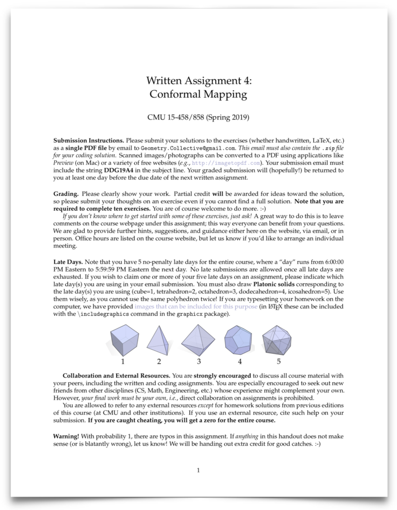
Assignment 4 [Written]: Conformal Parameterization (Due 4/18)

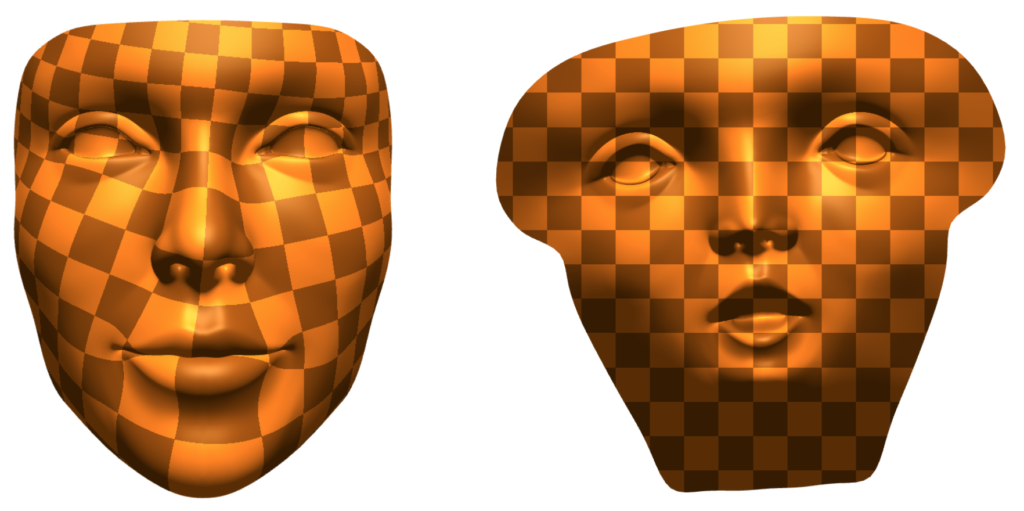
The written part of your next assignment, on conformal surface flattening, is now available below. Conformal flattening is important for (among other things) making the connection between processing of 3D surfaces, and existing fast algorithms for 2D image processing. You’ll have the opportunity to implement one of these algorithms in the coding part of the assignment.

Lecture 20: Discrete Conformal Geometry
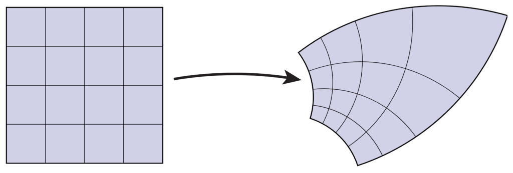
In this lecture we’ll attempt to translate several smooth characterizations of conformal maps into the discrete setting. We’ll also see how each of these attempts leads to a different class of computational algorithms, with different trade offs. Although conformal maps are often associated with angle preservation, we’ll see that preserving angles at the discrete level results in a theory that is far to rigid: i.e., it does not capture any of the interesting structure of smooth conformal geometry. Instead, we’ll see how less-obvious starting points (such as patterns of circles, or preservation of length cross ratios) lead to some deep and beautiful connections between the classic smooth picture, and the discrete, combinatorial picture.
