Lecture 19: Conformal Geometry

A basic task in geometric algorithms is finding mappings between surfaces, which can be used to transfer data from one place to another. A particularly nice class of algorithms (both from a mathematical and computational perspective) are conformal mappings, which preserve angles between vectors, and are generally very well-behaved. In this lecture we’ll take a look at smooth characterizations of conformal maps, which will ultimately inspire the way we talk about conformal maps in the discrete/computational setting.

Reading 6—The Laplace Operator (due March 30)

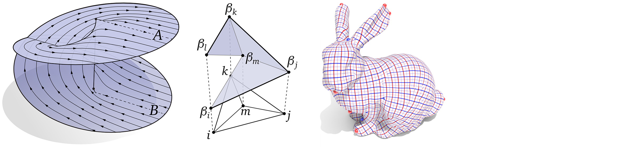
Your next reading covers one of the most fundamental objects in differential geometry, and one of the most useful objects in practical geometry processing: the Laplace-Beltrami operator \(\Delta\), which we’ll often refer to as just the “Laplacian”. This operator generalizes the familiar Laplace operator \(\Delta = \frac{\partial^2}{\partial x_1^2} + \cdots + \frac{\partial^2}{\partial x_n^2}\) from Euclidean \(\mathbb{R}^n\) to general curved manifolds. Like the ordinary Laplacian, at a very basic level Laplace-Beltrami provides information about the “curvature” of a function. It also shows up in an enormous number of physical and geometric equations, and for this reason there has been intense study of different ways to discretize the Laplacian (not only for simplicial meshes, but also point clouds and other discrete surface representations).

The reading will expose you to some of the key issues to think about when designing a discrete Laplacian. For this reading, you can choose either of the following two papers:

You should not worry about deeply understanding all of the mathematical details in these papers; the point is just to get a sense of the issues at stake, and how these considerations translate into practical definitions of discrete Laplace matrices. The first paper, by Wardetzky et al, considers a “No Free Lunch” theorem for discrete Laplacians that continues our story of “The Game” played in discrete differential geometry. The second paper, by Bobenko & Springborn considers the important perspective of intrinsic triangulations of polyhedral surfaces, and uses this perspective to develop a Laplace operator that is well-behaved even for very poor quality triangulations. You should simply summarize the high-level ideas in these papers, and any questions you might have.

The reading is due on Thursday, March 30 at 10am Eastern time. Hand-in instructions are as usual described on the assignments page.

Lectures 17 & 18—Laplace Beltrami

In the next two lectures we’ll take a deep dive into one of the most important objects not only in discrete differential geometry, but in differential geometry at large (not to mention physics!): the Laplace-Beltrami operator. This operator generalizes the familiar Laplacian you may have studied in vector calculus, which just gives the sum of second partial derivatives: \(\Delta \phi = \sum_i \partial^2 \phi_i / \partial x_i^2\). We’ll motivate Laplace-Beltrami from several points of view, talk about how to discretize it, and show how from a computational point of view it really is the —Swiss army knife— of geometry processing algorithms, essentially replacing the discrete Fourier transform from classical signal processing.

Lecture 16—Discrete Curvature II (Variational Viewpoint)

In this lecture we wrap up our discussion of discrete curvature, and see how it all fits together into a single unified picture that connects the integral viewpoint, the variational viewpoint, and the Steiner formula. Along the way we’ll touch upon several of the major players in discrete differential geometry, including a discrete version of Gauss-Bonnet, Schläfli’s polyhedral formula, and the cotan Laplace operator—which will be the focus of our next set of lectures.

Assignment 3 [Coding]: The Laplacian (Due 4/4)

For the coding portion of this assignment, you will build the so-called “cotan-Laplace” matrix and start to see how it can be used for a broad range of surface processing tasks, including the Poisson equation and two kinds of curvature flow.


Getting Started

Please implement the following routines in

  1. core/geometry.js:
    • laplaceMatrix
    • massMatrix
  2. projects/poisson-problem/scalar-poisson-problem.js:
    • constructor
    • solve
  3. projects/geometric-flow/mean-curvature-flow.js:
    • buildFlowOperator
    • integrate
  4. projects/geometric-flow/modified-mean-curvature-flow.js:
    • constructor
    • buildFlowOperator


Notes

  • Sections 6.4-6 of the course notes describe how to build the cotan-Laplace matrix and mass matrices, and outline how they can be used to solve equations on a mesh. In these applications you will be required to setup and solve a linear system of equations $Ax=b$ where $A$ is the Laplace matrix, or some slight modification thereof. Highly efficient numerical methods such as Cholesky Factorization can be used to solve such systems, but require A to be symmetric positive definite. Notice that the cotan-Laplace matrix described in the notes is negative semi-definite. To make it compatible for use with numerical methods like the Cholesky Factorization, your implementation of laplaceMatrix should instead produce a positive definite matrix, i.e., it should represent the expression
    $$(\Delta u)_i=\frac12 \sum_{ij}(\cot \alpha_{ij}+\cot \beta_{ij})(u_i–u_j).$$(Note that $u_i−u_j$ is reversed relative to the course notes.) To make this matrix strictly positive definite (rather than semidefinite), you should also add a small offset such as $10^{-8}$ to the diagonal of the matrix (which can be expressed in code as a floating point value 1e-8). This technique is known as Tikhonov regularization.
  • The mass matrix is a diagonal matrix containing the barycentric dual area of each vertex.
  • In the scalar Poisson problem, your goal is to discretize and solve the equation $\Delta \phi = \rho$ where $rho$ is a scalar density on vertices and $\Delta$ is the Laplace operator. Be careful about appropriately incorporating dual areas into the discretization of this equation (i.e., think about where and how the mass matrix should appear); also remember that the right-hand side cannot have a constant component (since then there is no solution).
  • In your implementation of the implicit mean curvature flow algorithm, you can encode the surface $f:M \to \mathbb R^3$ as a single DenseMatrix of size $|V| \times 3$, and solve with the same (scalar) cotan-Laplace matrix used for the previous part. When constructing the flow operator, you should follow section 6.6 of the notes. But be careful – when we discretize equations of the form $\Delta f = \rho$, we create systems of the form $A f = M \rho$. So you’ll need to add in the mass matrix somewhere. Also, recall that our discrete Laplace matrix is the negative of the actual Laplacian.
  • The modified mean curvature flow is nearly identical to standard mean curvature flow. The one and only difference is that you should not update the cotan-Laplace matrix each time step, i.e., you should always be using the cotans from the original input mesh. The mass matrix, however, must change on each iteration.

Submission Instructions

Please only turn in the source files geometry.[cpp|js], scalar-poisson-problem.[cpp|js], mean-curvature-flow.[cpp|js] and modified-mean-curvature-flow.[cpp|js] . These files should be submitted via the usual mechanism through gradescope.

The assignment is due on the date listed on the calendar, at 5:59:59pm Eastern (not at midnight!). Further hand-in instructions can be found on this page.

Assignment 3 [Written]: The Laplacian (Due 4/4)

These exercises will lead you through two different derivations for the cotan-Laplace operator. As we’ll discuss in class, this operator is basically the “Swiss army knife” of discrete differential geometry and digital geometry processing, opening the door to a huge number of interesting algorithms and applications. Note that this time the exercises all come from the course notes—you will need to read the accompanying notes in order to familiarize yourself with the necessary material (though actually we’ve covered much of this stuff in class already!)


Lecture 15—Discrete Curvature I (Integral Viewpoint)

Just as curvature provides powerful ways to describe and analyze smooth surfaces, discrete curvatures provide a powerful way to encode and manipulate digital geometry—and is a fundamental component of many modern algorithms for surface processing. This first of two lectures on discrete curvature from the integral viewpoint, i.e., integrating smooth expressions for discrete curvatures in order to obtain curvature formulae suitable for discrete surfaces. In the next lecture, we will see a complementary variational viewpoint, where discrete curvatures arise by instead taking derivatives of discrete geometry. Amazingly enough, these two perspectives will fit together naturally into a unified picture that connects essentially all of the standard discrete curvatures for triangle meshes.

Lecture 14—Smooth Curvature

Much of the geometry we encounter in everyday life (such as curves and surfaces sitting in space) is well-described by it curvatures. For instance, the fundamental theorem for plane curves says that an arc-length parameterized plane curve is determined by its curvature function, up to rigid motions. Similar statements can be made about surfaces and their curvatures, which we explore in this lecture.

Lecture 13—Discrete Surfaces

We’ll follow up our lecture on smooth surfaces with a view of surfaces from the discrete point of view. Our goal will be to translate basic concepts (such as the differential, immersions, etc.) into a purely discrete language. Here we’ll also start to see the benefit of developing discrete differential forms: many of the statements we made about surfaces in the smooth setting can be translated into the discrete setting with minimal effort. As we move forward with discrete differential geometry, this “easy translation” will enable us to take advantage of deep insights from differential geometry to develop practical computational algorithms.

Lecture 12—Smooth Surfaces

This lecture gives a crash course in the differential geometry of surfaces. There’s of course way more to know about surfaces than we can pack into a single lecture (and we’ll see plenty more later on), but this lecture will cover basic concepts like how to describe a surface and its normals. It also starts to connect surface theory to the other tools we’ve been building up, via vector-valued differential forms.