Category: Slides

In this lecture we’ll start taking a look at geodesics, which generalize the concept of a “straight line” to curved manifolds. Here again we encounter The Game of discrete differential geometry: different characterizations of geodesics—namely, straightest vs. (locally) shortest—will lead us down a path toward different discrete analogues, and ultimately, different algorithms.

In this lecture we’ll attempt to translate several smooth characterizations of conformal maps into the discrete setting. We’ll also see how each of these attempts leads to a different class of computational algorithms, with different trade offs. Although conformal maps are often associated with angle preservation, we’ll see that preserving angles at the discrete level results in a theory that is far to rigid: i.e., it does not capture any of the interesting structure of smooth conformal geometry. Instead, we’ll see how less-obvious starting points (such as patterns of circles, or preservation of length cross ratios) lead to some deep and beautiful connections between the classic smooth picture, and the discrete, combinatorial picture.

A basic task in geometric algorithms is finding mappings between surfaces, which can be used to transfer data from one place to another. A particularly nice class of algorithms (both from a mathematical and computational perspective) are conformal mappings, which preserve angles between vectors, and are generally very well-behaved. In this lecture we’ll take a look at smooth characterizations of conformal maps, which will ultimately inspire the way we talk about conformal maps in the discrete/computational setting.

In the next two lectures we’ll take a deep dive into one of the most important objects not only in discrete differential geometry, but in differential geometry at large (not to mention physics!): the Laplace-Beltrami operator. This operator generalizes the familiar Laplacian you may have studied in vector calculus, which just gives the sum of second partial derivatives: \(\Delta \phi = \sum_i \partial^2 \phi_i / \partial x_i^2\). We’ll motivate Laplace-Beltrami from several points of view, talk about how to discretize it, and show how from a computational point of view it really is the —Swiss army knife— of geometry processing algorithms, essentially replacing the discrete Fourier transform from classical signal processing.

In this lecture we wrap up our discussion of discrete curvature, and see how it all fits together into a single unified picture that connects the integral viewpoint, the variational viewpoint, and the Steiner formula. Along the way we’ll touch upon several of the major players in discrete differential geometry, including a discrete version of Gauss-Bonnet, Schläfli’s polyhedral formula, and the cotan Laplace operator—which will be the focus of our next set of lectures.

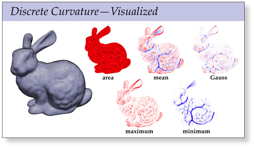
Just as curvature provides powerful ways to describe and analyze smooth surfaces, discrete curvatures provide a powerful way to encode and manipulate digital geometry—and is a fundamental component of many modern algorithms for surface processing. This first of two lectures on discrete curvature from the integral viewpoint, i.e., integrating smooth expressions for discrete curvatures in order to obtain curvature formulae suitable for discrete surfaces. In the next lecture, we will see a complementary variational viewpoint, where discrete curvatures arise by instead taking derivatives of discrete geometry. Amazingly enough, these two perspectives will fit together naturally into a unified picture that connects essentially all of the standard discrete curvatures for triangle meshes.

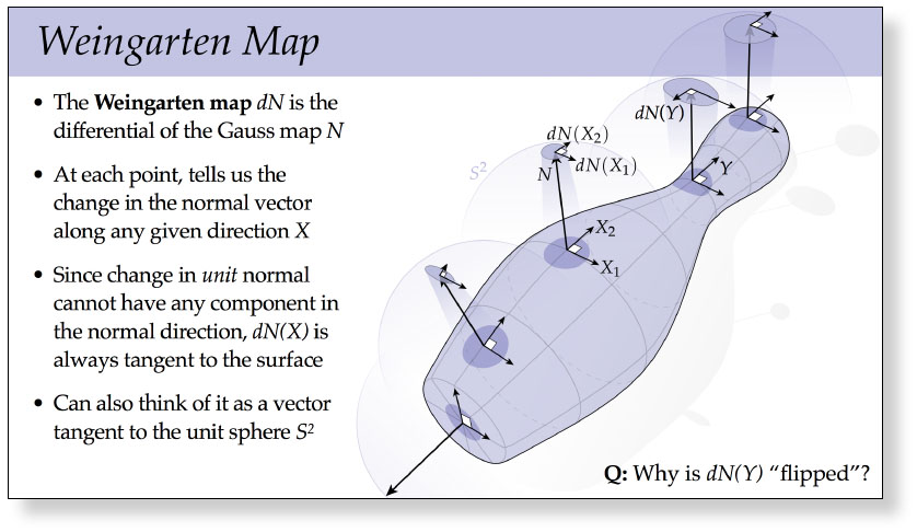
Much of the geometry we encounter in everyday life (such as curves and surfaces sitting in space) is well-described by it curvatures. For instance, the fundamental theorem for plane curves says that an arc-length parameterized plane curve is determined by its curvature function, up to rigid motions. Similar statements can be made about surfaces and their curvatures, which we explore in this lecture.

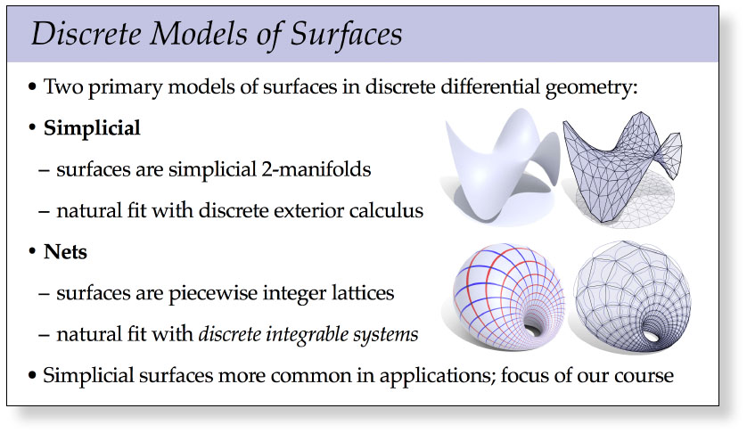
We’ll follow up our lecture on smooth surfaces with a view of surfaces from the discrete point of view. Our goal will be to translate basic concepts (such as the differential, immersions, etc.) into a purely discrete language. Here we’ll also start to see the benefit of developing discrete differential forms: many of the statements we made about surfaces in the smooth setting can be translated into the discrete setting with minimal effort. As we move forward with discrete differential geometry, this “easy translation” will enable us to take advantage of deep insights from differential geometry to develop practical computational algorithms.

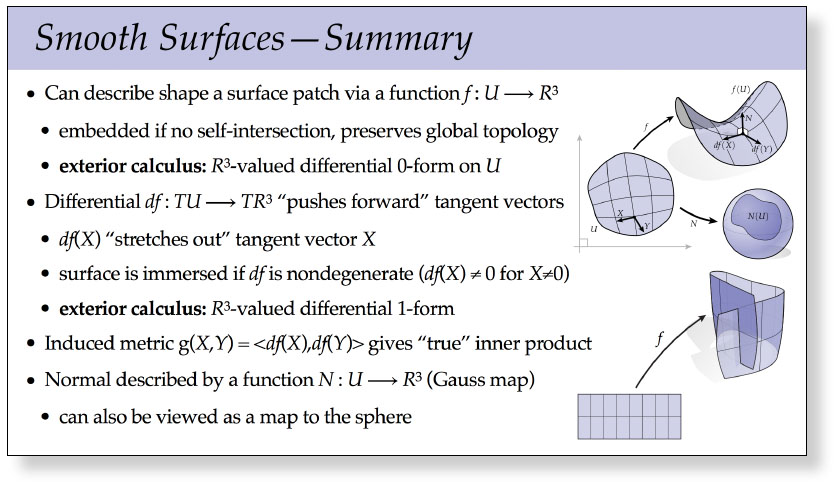
This lecture gives a crash course in the differential geometry of surfaces. There’s of course way more to know about surfaces than we can pack into a single lecture (and we’ll see plenty more later on), but this lecture will cover basic concepts like how to describe a surface and its normals. It also starts to connect surface theory to the other tools we’ve been building up, via vector-valued differential forms.

This lecture presents the discrete counterpart of the previous lecture on smooth curves. Here we also arrive at a discrete version of the fundamental theorem for plane curves: a discrete curve is completely determined by its discrete parameterization (a.k.a. edge lengths) and its discrete curvature (a.k.a. exterior angles). Can you come up with a discrete version of the fundamental theorem for space curves? If we think of torsion as the rate at which the binormal is changing, then a natural analogue might be to (i) associate a binormal \(B_i\) with each vertex, equal to the normal of the plane containing \(f_{i-1}\), \(f_{i}\), and \(f_{i+1}\), and (ii) associate a torsion \(\tau_{ij}\) to each edge \(ij\), equal to the angle between \(B_i\) and \(B_{i+1}\). Using this data, can you recover a discrete space curve from edge lengths \(\ell_{ij}\), exterior angles \(\kappa_i\) at vertices, and torsions \(\tau_{ij}\) associated with edges? What’s the actual algorithm? (If you find this problem intriguing, leave a comment in the notes! It’s not required for class credit.)