The written portion of Assignment 2 can be found below. It takes a look at the curvature of smooth and discrete surfaces, which we have been talking about in lecture.

CS 15-458/858: Discrete Differential Geometry
CARNEGIE MELLON UNIVERSITY | SPRING 2023 | TUE/THU 12:30-1:50 | GHC 4303
The written portion of Assignment 2 can be found below. It takes a look at the curvature of smooth and discrete surfaces, which we have been talking about in lecture.
For the coding portion of this assignment, you will implement various expressions for discrete curvatures and surfaces normals that you will derive in the written assignment. (However, the final expressions are given below in case you want to do the coding first.) Once implemented, you will be able to visualize these geometric quantities on a mesh. For simplicity, you may assume that the mesh has no boundary.
Getting Started
Please implement the following routines in core/geometry.[js/cpp]:
Notes
1. The dihedral angle between the normals $N_{ijk}$ and $N_{ijl}$ of two adjacent faces $ijk$ and $ijl$ (respectively) is given by
$$ \theta_{ij} := \text{atan2}\left(\frac{e_{ij}}{\|e_{ij}\|} \cdot \left(N_{ijk} \times N_{jil}\right), N_{ijk} \cdot N_{jil}\right)$$
where $e_{ij}$ is the vector from vertex $i$ to vertex $j$.
2. The formulas for the angle weighted normal, sphere inscribed normal, area weighted normal, discrete Gaussian curvature normal and discrete mean curvature normal at vertex $i$ are
\[\begin{aligned}
N_i^\phi &:= \sum_{ijk \in F} \phi_i^{jk}N_{ijk}\\
N_i^S &:= \sum_{ijk \in F} \frac{e_{ij} \times e_{ik}} {\|e_{ij}\|^2\|e_{ik}\|^2}\\
N_i^A &:= \sum_{ijk \in F} A_{ijk}N_{ijk}\\
KN_i &= \frac 12 \sum_{ij \in E} \frac{\theta_{ij}}{\|e_{ij}\|}e_{ij}\\
HN_i &= \frac 12 \sum_{ij \in E}\left(\cot\left(\alpha_k^{ij}\right) + \cot\left(\beta_l^{ij}\right)\right)e_{ij}
\end{aligned}
\]
where $\phi_i^{jk}$ is the interior angle between edges $e_{ij}$ and $e_{ik}$, and $A_{ijk}$ is the area of face $ijk$. Note that sums are taken only over elements (edges or faces) containing vertex $i$. Normalize the final value of all your normal vectors before returning them.
3. The circumcentric dual area at vertex $i$ is given by
\[A_i := \frac 18 \sum_{ijk \in F} \|e_{ik}\|^2\cot\left(\alpha_j^{ki}\right) + \|e_{ij}\|^2\cot\left(\beta_k^{ij}\right)\]
4. The discrete scalar Gaussian curvature (also known as angle defect) and discrete scalar mean curvature at vertex $i$ are given by
\[\begin{aligned}
K_i &:= 2\pi – \sum_{ijk \in F} \phi_i^{jk}\\
H_i &:= \frac 12 \sum_{ij \in E} \theta_{ij}\|e_{ij}\|
\end{aligned}
\]
Note that these quantities are discrete 2-forms, i.e., they represent the total Gaussian and mean curvature integrated over a neighborhood of a vertex. They can be converted to pointwise quantities (i.e., discrete 0-forms at vertices) by dividing them by the circumcentric dual area of the vertex (i.e., by applying the discrete Hodge star).
5. You are required to derive expressions for the principal curvatures $\kappa_1$ and $\kappa_2$ in exercise 4 of the written assignment. Your implementation of principalCurvatures should return the (pointwise) minimum and maximum principal curvature values at a vertex (in that order).
Submission Instructions
Please submit only the source code file geometry.js or geometry.cpp (depending on whether you’re using JavaScript or C++). This means your code should not depend on edits made to any other files. Then follow the usual hand-in instructions.
The assignment is due on the date listed on the calendar, at 5:59:59pm Eastern (not at midnight!). Further hand-in instructions can be found on this page.
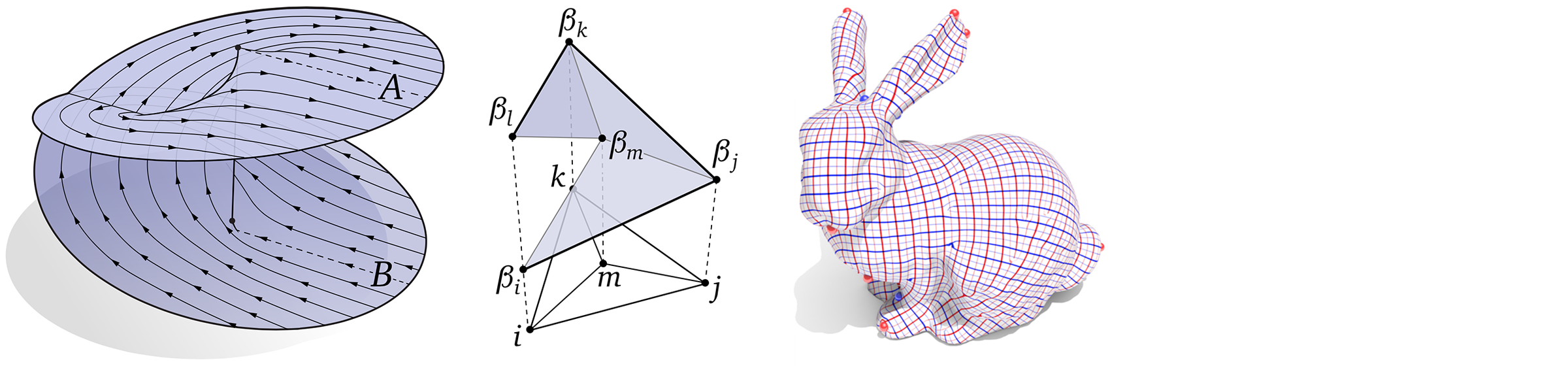
This lecture presents the discrete counterpart of the previous lecture on smooth curves. Here we also arrive at a discrete version of the fundamental theorem for plane curves: a discrete curve is completely determined by its discrete parameterization (a.k.a. edge lengths) and its discrete curvature (a.k.a. exterior angles). Can you come up with a discrete version of the fundamental theorem for space curves? If we think of torsion as the rate at which the binormal is changing, then a natural analogue might be to (i) associate a binormal \(B_i\) with each vertex, equal to the normal of the plane containing \(f_{i-1}\), \(f_{i}\), and \(f_{i+1}\), and (ii) associate a torsion \(\tau_{ij}\) to each edge \(ij\), equal to the angle between \(B_i\) and \(B_{i+1}\). Using this data, can you recover a discrete space curve from edge lengths \(\ell_{ij}\), exterior angles \(\kappa_i\) at vertices, and torsions \(\tau_{ij}\) associated with edges? What’s the actual algorithm? (If you find this problem intriguing, leave a comment in the notes! It’s not required for class credit.)
![]()
After spending a great deal of time understanding some basic algebraic and analytic tools (exterior algebra and exterior calculus), we’ll finally start talking about geometry in earnest, starting with smooth plane and space curves. Even low-dimensional geometry like curves reveal a lot of the phenomena that arise when studying curved manifolds in general. Our main result for this lecture is the fundamental theorem of space curves, which reveals that (loosely speaking) a curve is entirely determined by its curvatures. Descriptions of geometry in terms of “auxiliary” quantities such as curvature play an important role in computation, since different algorithms may be easier or harder to formulate depending on the quantities or variables used to represent the geometry. Next lecture, for instance, we’ll see some examples of algorithms for curvature flow, which naturally play well with representations based on curvature!
![]()
This lecture wraps up our discussion of discrete exterior calculus, which will provide the basis for many of the algorithms we’ll develop in this class. Here we’ll encounter the same operations as in the smooth setting (Hodge star, wedge product, exterior derivative, etc.), which in the discrete setting are encoded by simple matrices that translate problems involving differential forms into ordinary linear algebra problems.
![]()
The written portion of assignment 1 is now available, which covers some of the fundamental tools we’ll be using in our class. Initially this assignment may look a bit intimidating, but the homework is not as long as it might seem: all the text in the big gray blocks contains supplementary, formal definitions that you do not need to know in order to complete the assignments.
Finally, don’t be shy about asking us questions here in the comments, via email, or during office hours. We want to help you succeed on this assignment, so that you can enjoy all the adventures yet to come…
This assignment is due on Tuesday, February 28 at 5:59:59pm Eastern (not at midnight!).
![]()
For the coding portion of your first assignment, you will implement the discrete exterior calculus (DEC) operators $\star_0, \star_1, \star_2, d_0$ and $d_1$. Once implemented, you will be able to apply these operators to a scalar function (as depicted above) by pressing the “$\star$” and “$d$” button in the viewer. The diagram shown above will be updated to indicate what kind of differential k-form is currently displayed. These basic operations will be the starting point for many of the algorithms we will implement throughout the rest of the class; the visualization (and implementation!) should help you build further intuition about what these operators mean and how they work
Getting Started
In practice, a simple and efficient way to compute the cotangent of the angle $\theta$ between two vectors $u$ and $v$ is to use the cross product and the dot product rather than calling any trigonometric functions directly; we ask that you implement your solution this way. (Hint: how are the dot and cross product of two vectors related to the cosine and sine of the angle between them?)
In case we have not yet covered it in class, the barycentric dual area associated with a vertex $i$ is equal to one-third the area of all triangles $ijk$ touching $i$.
EDIT: You can compute the ratio of dual edge lengths to primal edge lengths using the cotan formula, which can be found on Slide 28 of the Discrete Exterior Calculus lecture, or in exercise 36 of the notes (you don’t have to do the exercise for this homework).
Submission Instructions
Please submit your geometry.[js|cpp] and discrete-exterior-calculus.[js|cpp] files to Gradescope. You should not submit any other source files (and therefore, should not edit any other source files to get your code working!).
The assignment is due on the date listed on the calendar, at 5:59:59pm Eastern (not at midnight!). Further hand-in instructions can be found on this page.
In this lecture, we turn smooth differential \(k\)-forms into discrete objects that we can actually compute with. The basic idea is actually quite simple: to capture some information about a differential \(k\)-form, we integrate it over each oriented \(k\)-simplex of a mesh. The resulting values are just ordinary numbers that give us some sense of what the original \(k\)-form must have looked like.
![]()
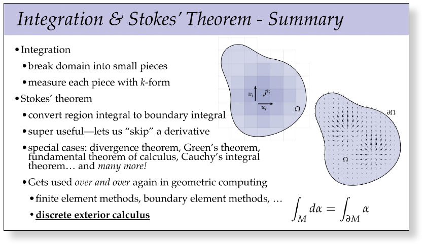
The next reading assignment will wrap up our discussion of exterior calculus, both smooth and discrete. In particular, it will explore how to differentiate and integrate \(k\)-forms, and how an important relationship between differentiation and integration (Stokes’ theorem) enables us to turn derivatives into discrete operations on meshes. In particular, the basic data we will work with in the computational setting are “integrals of derivatives,” which amount to simple scalar quantities we can associate with the vertices, edges, faces, etc. of a simplicial mesh. These tools will provide the basis for the algorithms we’ll explore throughout the rest of the semester.
The reading is the remainder of Chapter 4 from the course notes, “A Quick and Dirty Introduction to Exterior Calculus”, Sections 4.6 through 4.8 (pages 67–83). Note that you just have to read these sections; you do not have to do the written exercises; a different set of written problems will be posted later on. The reading is due Thursday, February 16 at 10am. See the assignments page for handin instructions.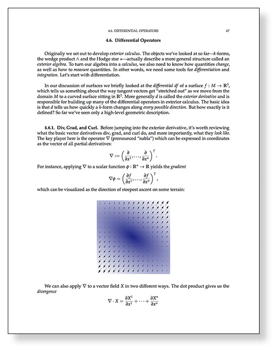
Our first lecture on exterior calculus covered differentiation; our second lecture completes the picture by discussing integration of differential forms. The relationship between integration and differentiation is encapsulated by Stokes’ theorem, which generalizes the fundamental theorem of calculus, as well as many other important theorems from vector calculus and complex analysis (divergence theorem, Green’s theorem, Cauchy’s integral formula, etc.). Stokes’ theorem also plays a key role in numerical discretization of geometric problems, appearing for instance in finite volume methods and boundary element methods; for us it will be the essential tool for developing a discrete version of differential forms that we can actually compute with.